◮ Ethereum Price Prediction with LSTM

The time series aspect of time series data can feel like a bit of a hurdle to jump over, and predicting stock and crypto prices is a whole other time series beast to tame. So in this article, I will walk you through the steps of creating a basic architecture to do just that. While this project does not give away any amazing secrets to prediction to the extent that you will become a millionaire overnight (I will be keeping those to myself), it does give you the overall structure to try out your ideas and feature engineering and see if you can do just that! So let's get started!

In this project, I am working with PyTorch and PyTorch Lightning and creating an LSTM neural network model.  I will go over the basic steps of using the PyTorch Lightning module on top of the PyTorch steps for this process. PyTorch Lightning is somewhat new to me, and I must be honest and admit that I am not completely sold on its usefulness just yet. The jury is still out. But by following along, you can see the steps, get an overall idea of how it works, and then you will be able to try it out for with your own projects and see what you think.

Please keep in mind this is not an endorsement of ethereum, nor is it a suggestion that you invest in ethereum.

1. Compile Stocks

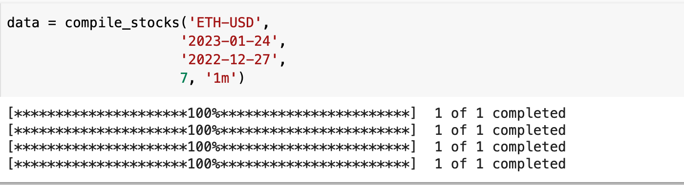
My crypto of choice is ethereum. So for this project, we will be importing as much minute-by-minute data for ethereum as possible, going backward from today, which as of the time I am writing this is, January 24, 2023. I will be using Yahooo Finance and the yfinance libray to import the data. Yahoo Finance only allows seven days worth of data at one minute intervals for a single import, and unfortunately, they also only allow a thirty day history of one minute interval data.

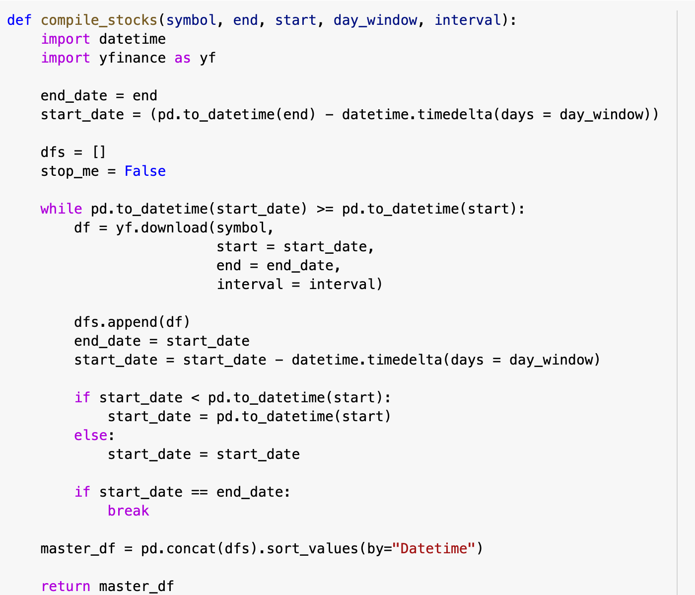
To make this easier and to work around the Yahoo Finance limitations, I wrote the following function which will compile dataframes in seven day increments for an entire range of dates so that the entire data will be the last month of ethereum prices at one minute intervals.

compile_stocks() takes the ticker symbol and the the end and start date, as well as the day_window, which in this case, as dictated by Yahoo Finance, is seven days. Then it also takes the interval, which in this case is one minute.

It downloads the most recent seven days, then calcuates the dates for the seven days prior and then downloads that data, repeating those steps until it goes all the way back to the start date requested. It then concatenates the dataframes it has collected into a single dataframe and sorts all of the data by the date column, which is its index. This function could be easily customized to work with other APIs that have such limitations on the download of data.

2. The Data

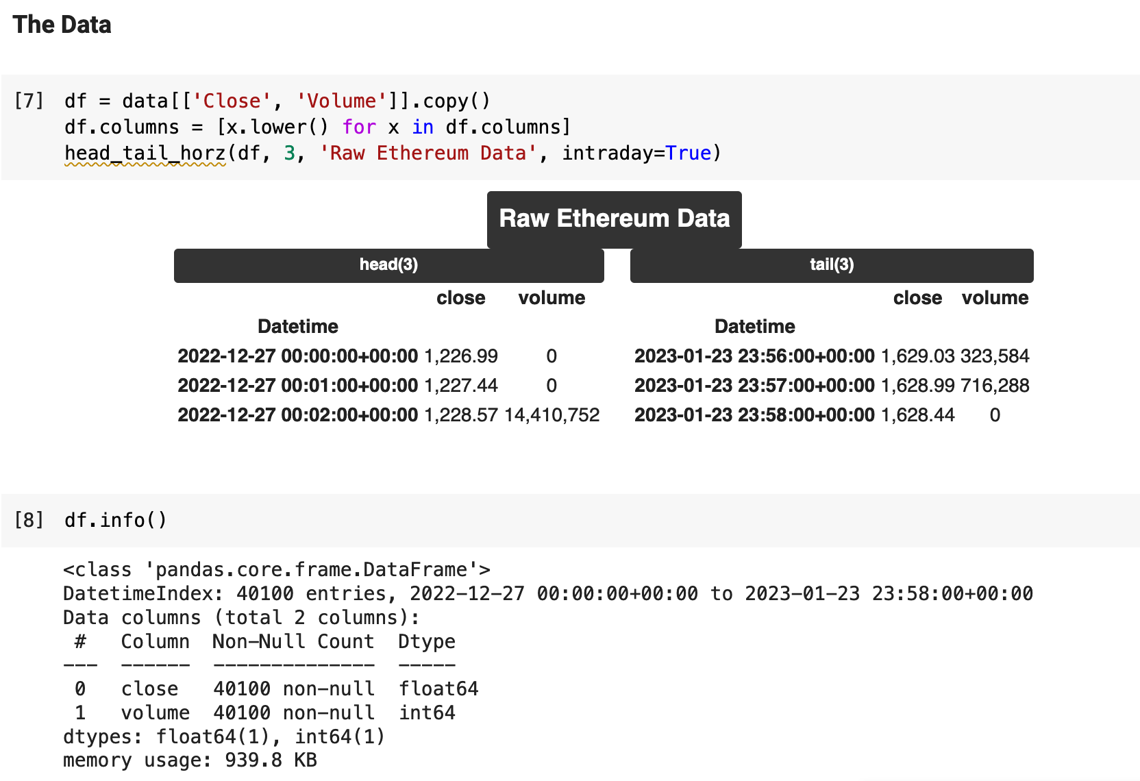
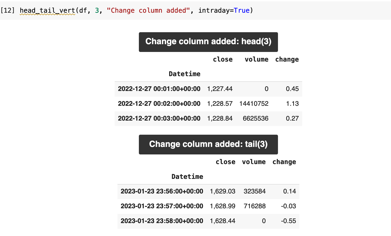
With the data downloaded and concatenated into a nice, clean dataframe, we can start to investigate. There are only 40,100 records in the dataset, which I found to be disappointing. So I am currently looking into the best options for acquiring more extensive and comprehensive data. Check back soon for more on the topic! For now, we will work with what we have. It is certainly enough to get somewhere and use for exhibiting the process of building a time series, price-prediction project.

I chose to only keep the close and volume columns from the original data, because the open, high, low, and adjusted close columns made no difference in the outcome, as I had worked with all the data including those columns previously with no change in results.  I could see no reason to keep data and run computations that are essentially useless.

3. Feature Engineering

These are just a few simple ideas of  features that can be added easily and quickly to any stock price prediction project. The first feature I added was a column that contains the value of the difference from the previous timestamp to the current. I do this using the shift() method in Pandas, create a temporary column containing the previous timestamp's price, then create the new change column by subtracting the previous timestamp's price from the current one. I then delete the temporary column with the previous value.

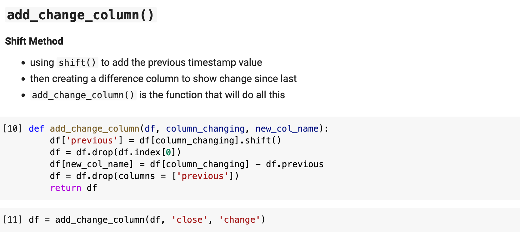
This now creates a quick way to read over the data and see, for example, where there are negative changes in the price versus positive. It also makes it easy to quickly see where there were more significant shifts in price.

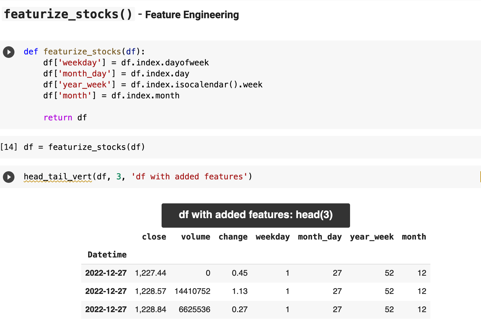
The next features I added were all related to the date: the day of the week, the day of the month, the year of the week, and the month of the year. While these are not incredibly informative, I decided to add them just to see if they give the model new opportunities for creating more accurate predictions.

With Pandas, adding these four new features is incredibly easy and quick, as you can see below. It can be done in just a few short lines of code. I must admit, I have seen plenty of others iterate over entire dataframes to do this. And honestly, I find it painful to read such code, let alone imagine how much longer it must take to run the code when a dataset is several million records long. It is very important to always take advantage of the vector-driven power that Pandas offers. And the code is far more beautiful this way.  Just remember: friends don't let friends interrows().

4. Splitting and Scaling the Data

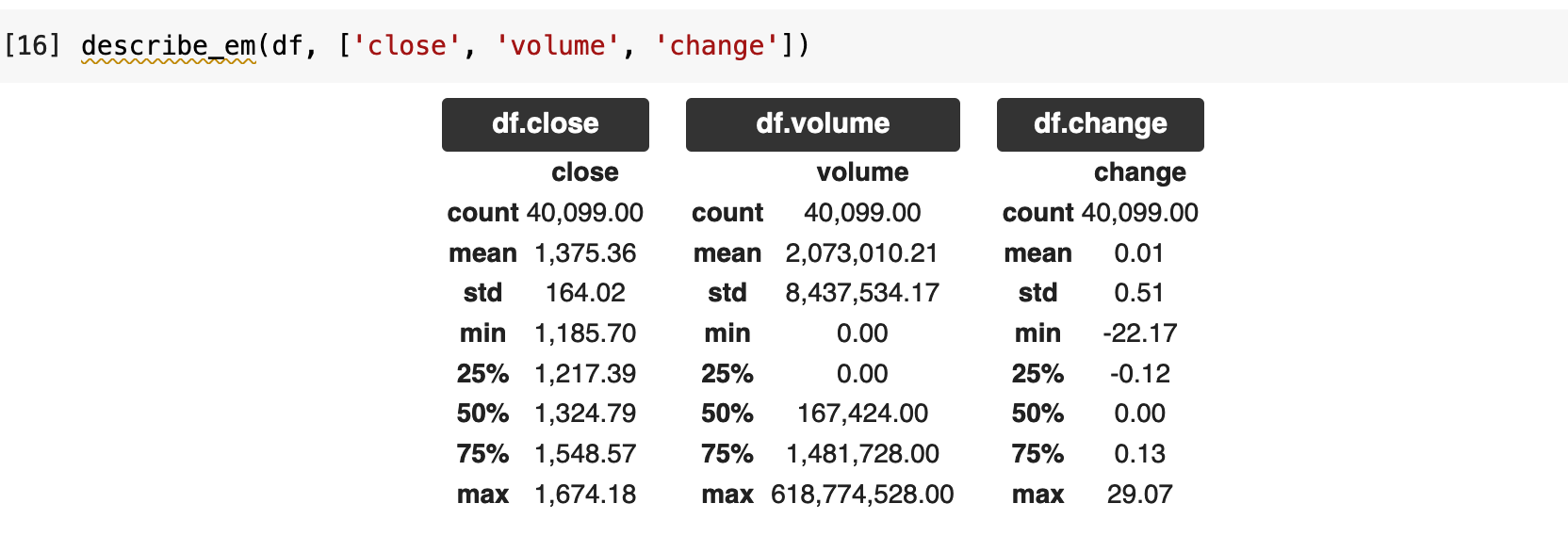
Before splitting and scaling, I like to get a final look at the describe method for the data and keep an overall image in my mind of my data. Once it is scaled and we are working with datasets and dataloaders, things change. So this is my farewell to the more human-comprehensible version of my data before translating to model-speak.

I like to see the main features and their distributions separated out, as it helps me to quickly capture a mental image and comprehend the overall structure of the data. So I wrote this little function called describe_em(), which will take the dataframe and a list of columns and separate out their describe() outputs individually.

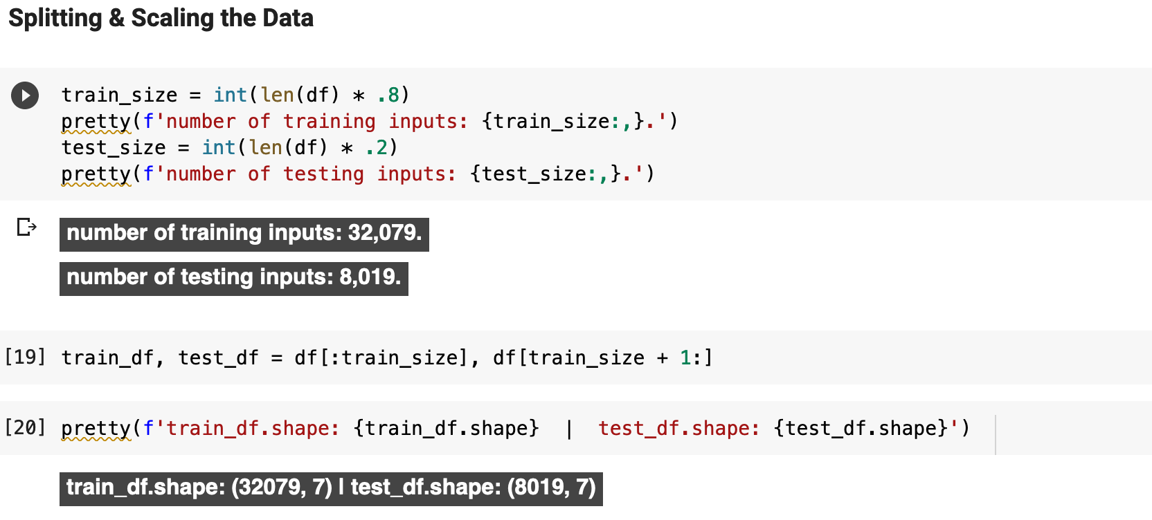
With time series data, especially when attempting to accurately predict stock and crypto prices, it is very important to split the data appropriately. For the split, I used 80% for training and the last 20% for testing and predicting, the most recent 20% being the testing data. The following shows the number of resulting record for the training and testing sets. You can also see here the shape of our data, which has seven columns, or features. Price preditction time series data is awkward in the sense that we are using the same column, close, in our input data as a feature even though it is technically also our target data. We will look into this relationship more deeply when we get to the section discussing the creation of sequences for training.

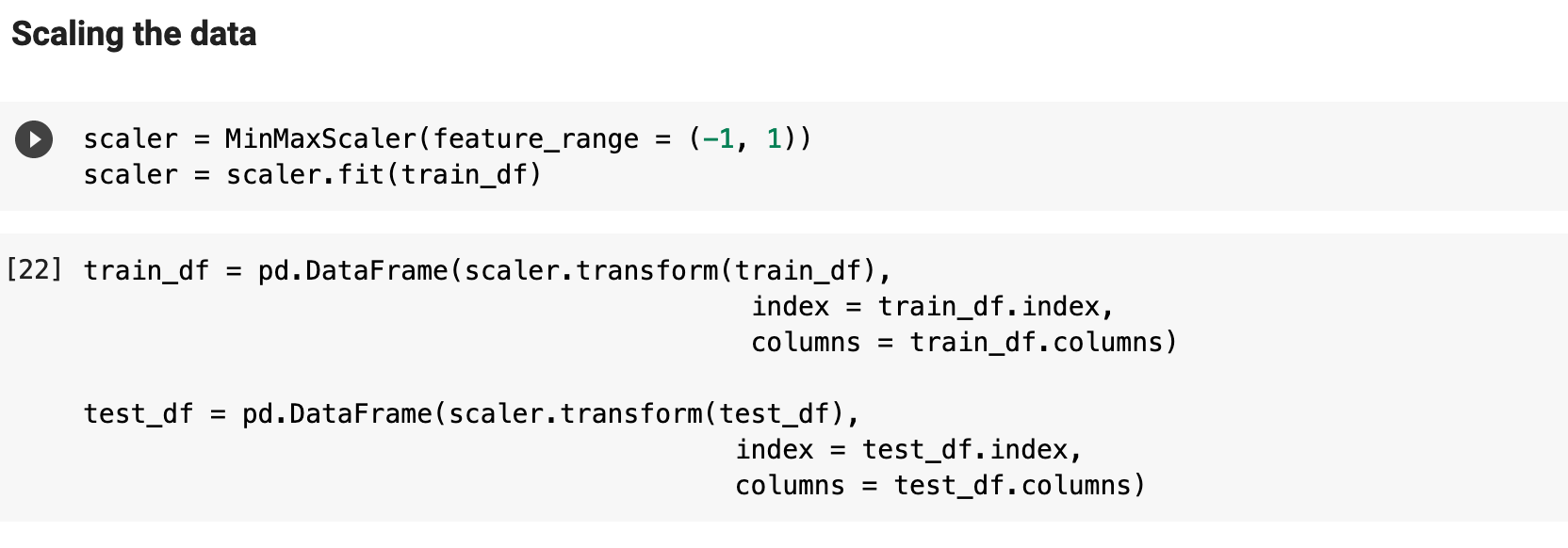
I use the scikit-learn MinMaxScaler() for scaling the data and use the range (-1, 1).  Here I am applying this scaling to the newly created split dataframes, train_df and test_df.

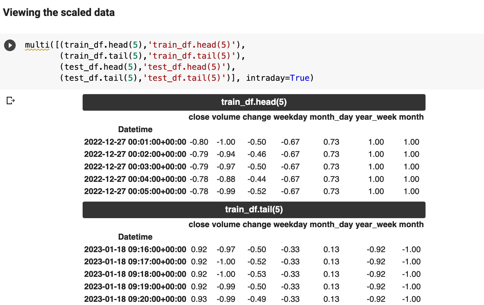
And here we get a view of the data now that it is scaled.

5. Creating the Sequences

This is when it gets fun. When working with stock and crypto price prediction, it is customary to follow the following steps:

• create sequences
• convert sequences to datasets
• convert datasets to dataloaders
• feed dataloaders to the model

In the testing phase, the sequences serve as the inputs for each of our predictions. For example, in this project, my sequences are 60 timestamps in length, each timestamp being at one minute intervals, thus a sequence covers one hour. For each sequence, we get a prediction for the next timestamp's price. Think of it like a sliding window of length 60, which moves across the data. At each point, from the beginning to the end of our training data, we have a label for each individual collection of 60 consecutive data points, then we move the window up by one spot, which has its label, and so on. Consequently, we will have sequences totaling the length of the data minus the length of one sequence, since the first records can only be used once for the first sequence and its label. If this is confusing, do not worry. I have examples below!

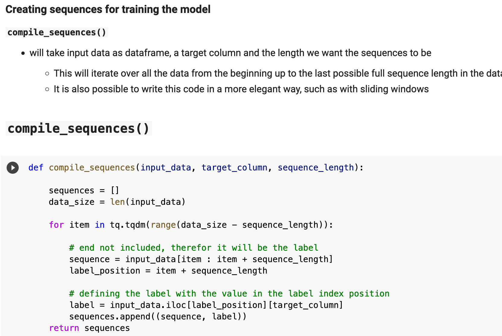
The function compile_sequences() takes the input data, the training dataframe and the testing dataframe, and performs the previously described operation. The target column is the name of the column where we will be getting the label every time we move the window forward. And the sequence length, in our case, is the number of timestamps to group together and give a label to.

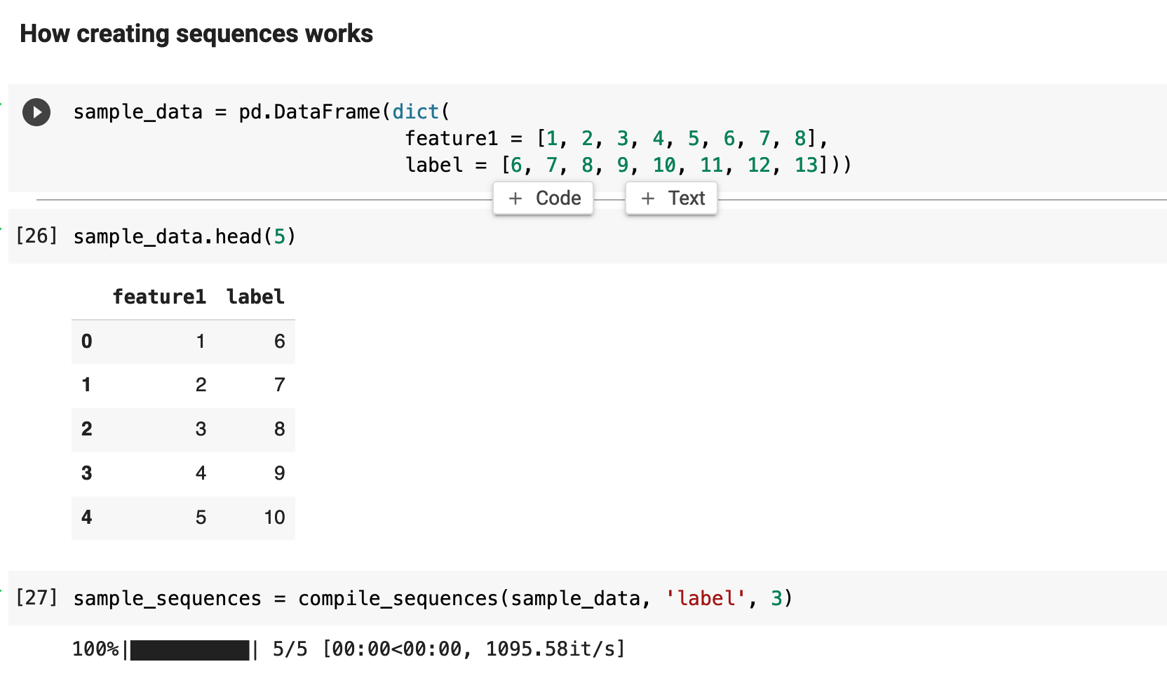
Let's look at how this process of working with sequences actually works. The sample data below is merely a collection of integers, one serving as a feature column, and one named "label". We could group these records in sequences of length 2, 3, 4, and that's about it. Because we do not have much data here.

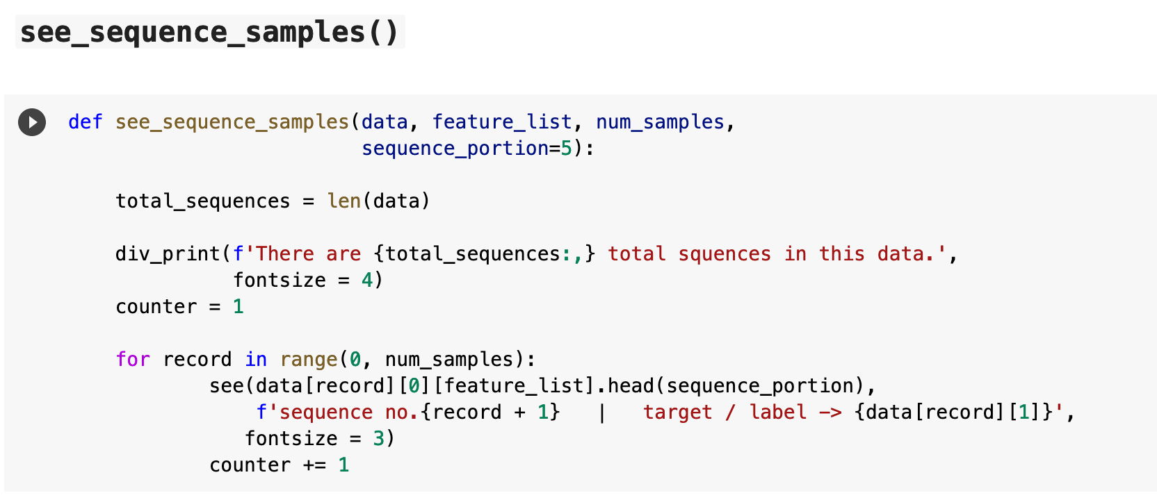
The following function will produce sequences and their labels to make this process more clear. see_sequence_samples() takes the data, the features to be sequenced, the number of samples we want output, and how much of the sequence we want to see each output. For example, our training and testing sequences will be 60 records in length each. We probably do not want to print the entirety of a sequence in that case, but rather a portion of a sequence, just to check our data.  So I have set the default to five records per sequence.

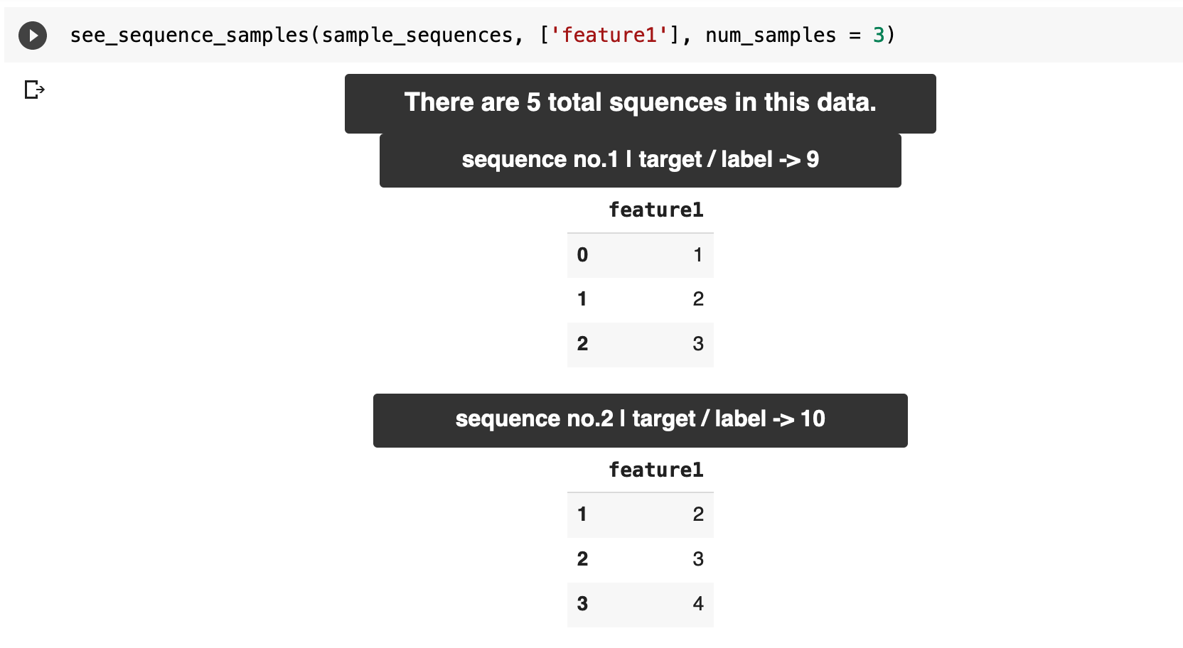
Here, we are getting sequence samples from our sample data above. First, we get the total number of sequences that has been made from our data and given the sequence length, then we get our example sequences with the label for each in the header for each. So sequence number 1 has inputs of 1, 2, and 3. And the correct label for this data is 9.  Then sequence number 2 has the label 10, and so on.

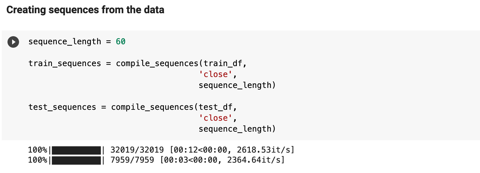
The following is compiling the sequences for our actual training and testing data. This is where we decide on the sequence length. And I pass the close column as the column from which to gather the label for each sequence.

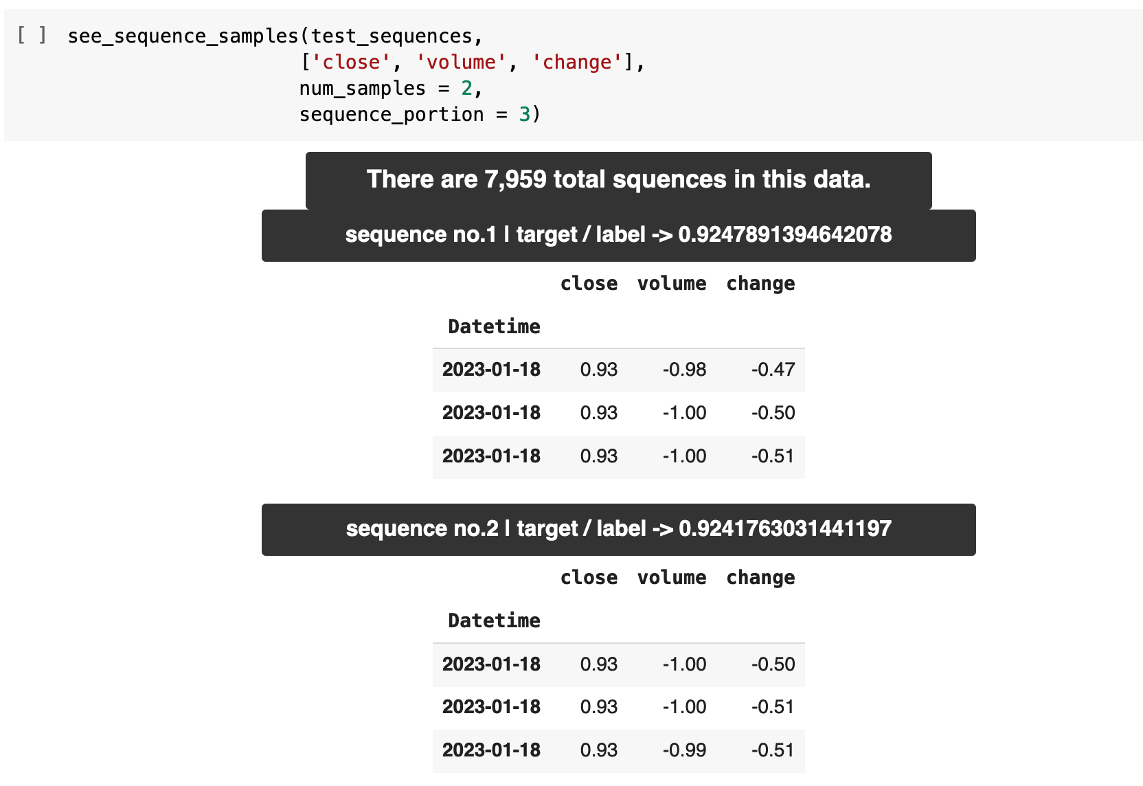
Here we see some samples of our sequences for the training data and the testing data. For every grouping of 60 records of data, the label for that data will be the value in the close column for the record at the 61st spot in the data, relative to the current position within the data.

One way to conceptualize this is to imagine that for every window of 60 minutes worth of values (60 individual timestamps as a sequence), we get the ethereum price that comes at the record just following, thus the result of the previous 60 that led up to it.

6. Creating the Datasets

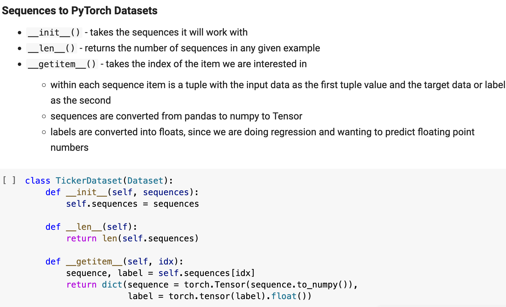
Much of the explanation for the following steps is contained within the markdown cells accompanying my code in my Jupyter notebook excerpts below. I attempt to thoroughly explain each step and aspect of the process for as complete a comprehension as possible. The first step is to instantiate the PyTorch Dataset class, which I have named TickerDataset. This structure can be used with just about any stock ticker data.

The thing about PyTorch Lightning is: it adds a fair number of extra steps to the entire process, which can be very useful if you know how to utilize them to their fullest.  The way they describe it on the front page of the website is "Spend more time on research, less on engineering." I honestly cannot say if they succeeded in making that a reality, as I felt like it possibly caused me to spend MORE time on the engineering of the entire project.  But this is not something I mind. I actually very much enjoy that part of the process. Alas, I will delay final judgement on PyTorch Lightning's utility, however, until I have worked with the library more and can give a fair and justified opinion on the process as a whole.

The majority of the benefit of the following extra steps comes in later during the training portion, when we are able to utilize checkpoints, early stopping, and other benefits of the library. And I must admit that those features are quite nice. So keep in mind that there will be pay off for these extra steps in the process.

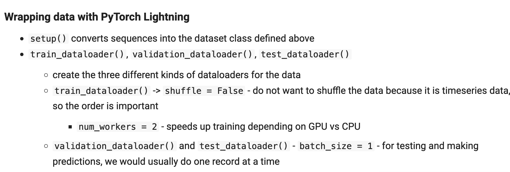
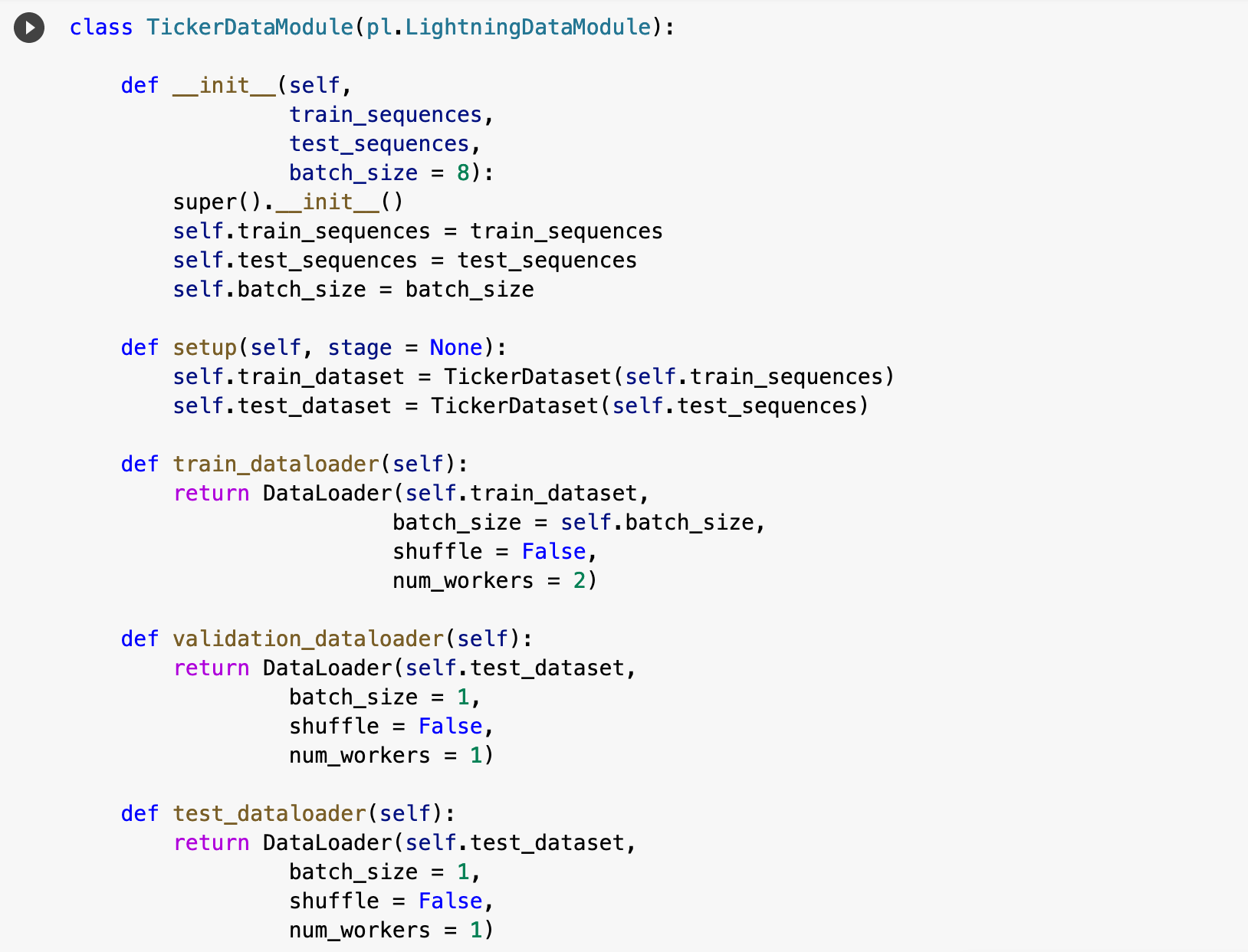
The following is essentially the PyTorch Lightning way of creating the class for the PyTorch dataloaders for the training, validation, and testing portions of the project. Note: I will not be using the validation step.

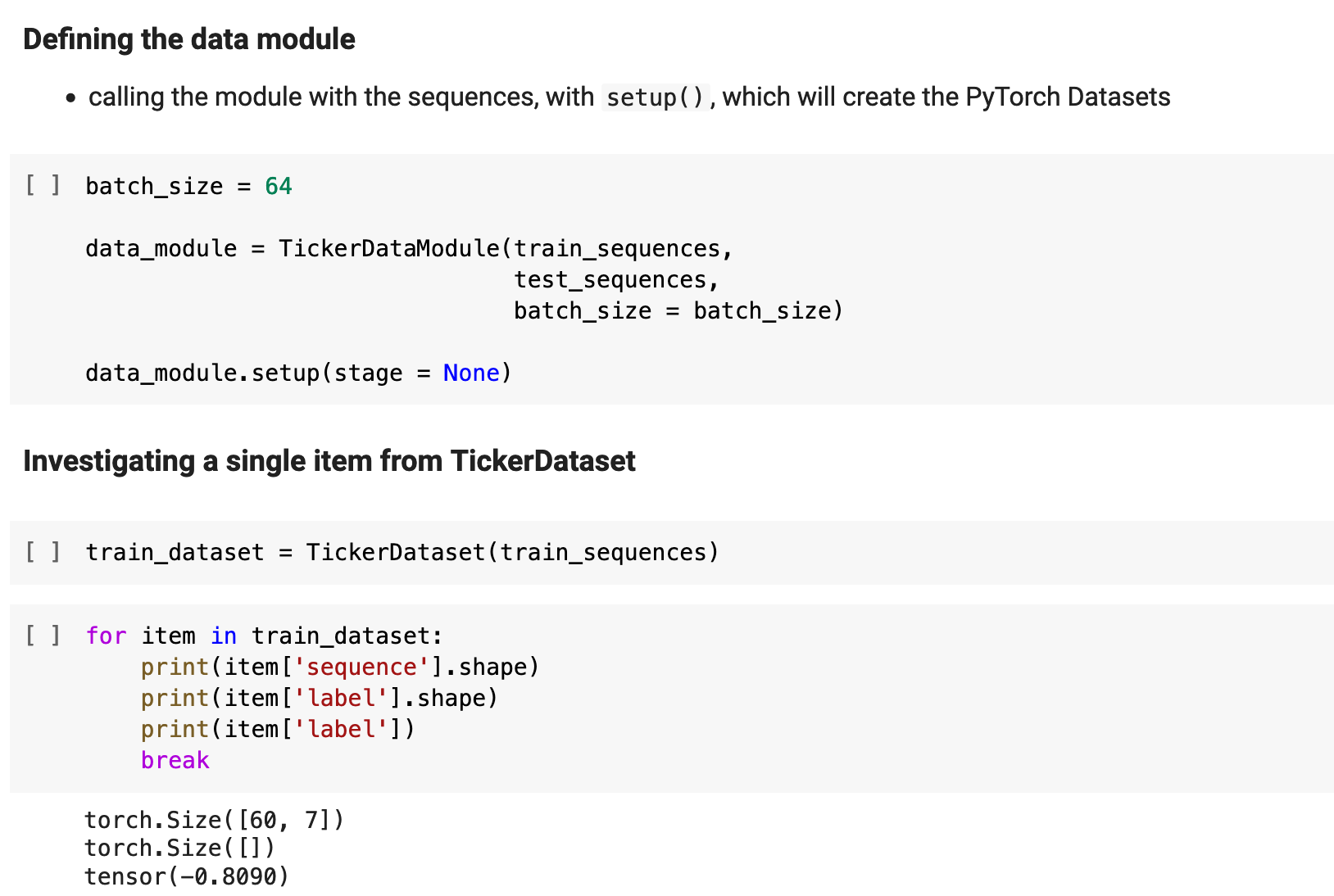
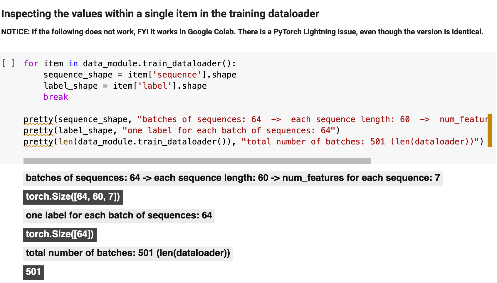
And here I put all of this together and apply it all to the data, creating the training dataset. And below, I check an example from the resulting dataset just to be sure that our shapes and datatypes are correct.

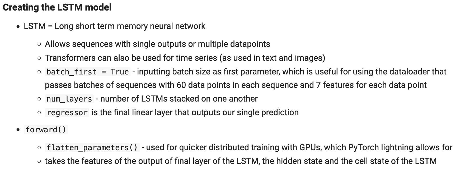
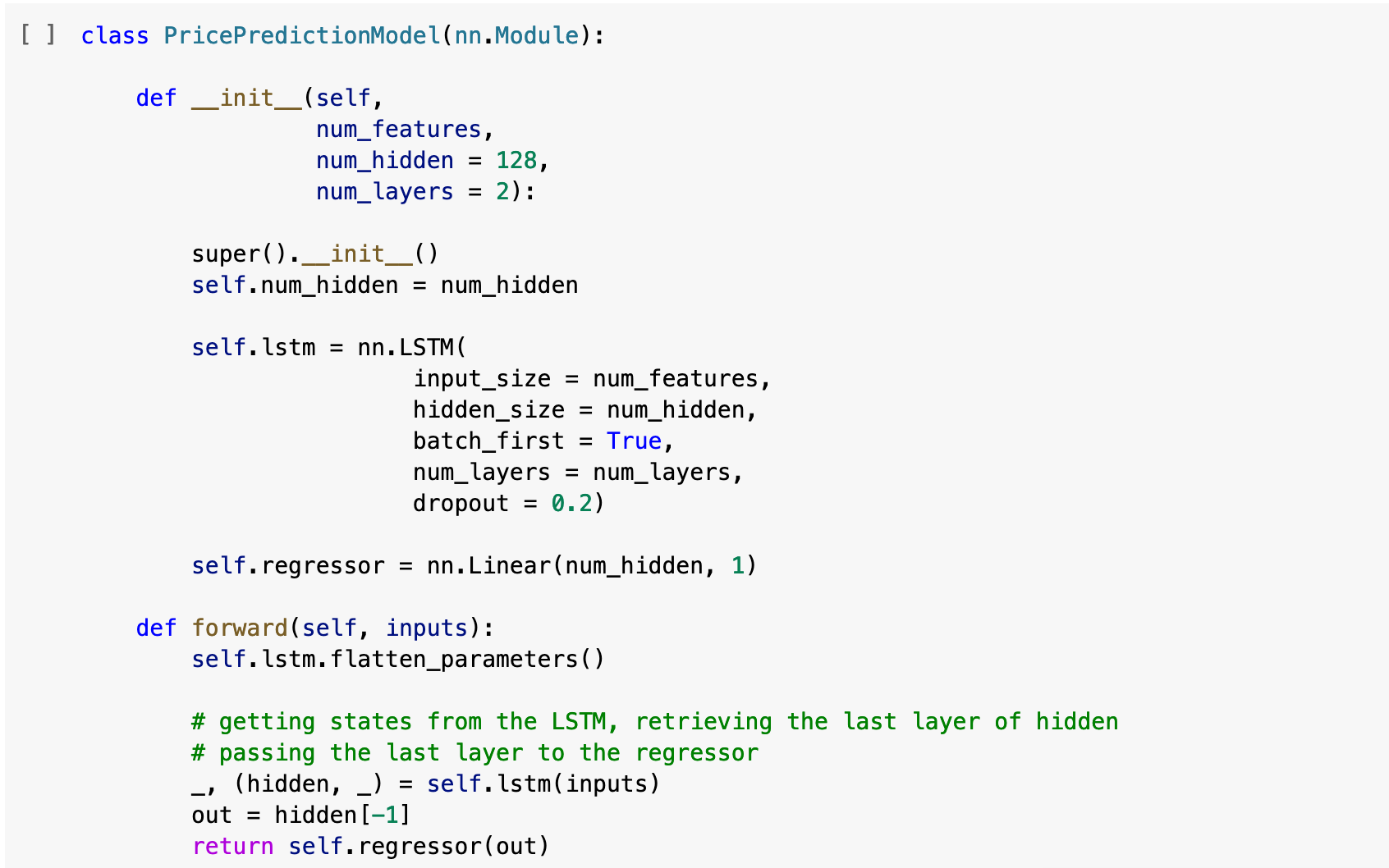
7. The LSTM Model

Now for the creation of the model. This follows a typical PyTorch method of defining the model class. I have chosen to use 128 hidden layers and 2 LSTM layers for my model with a dropout rate of 20%

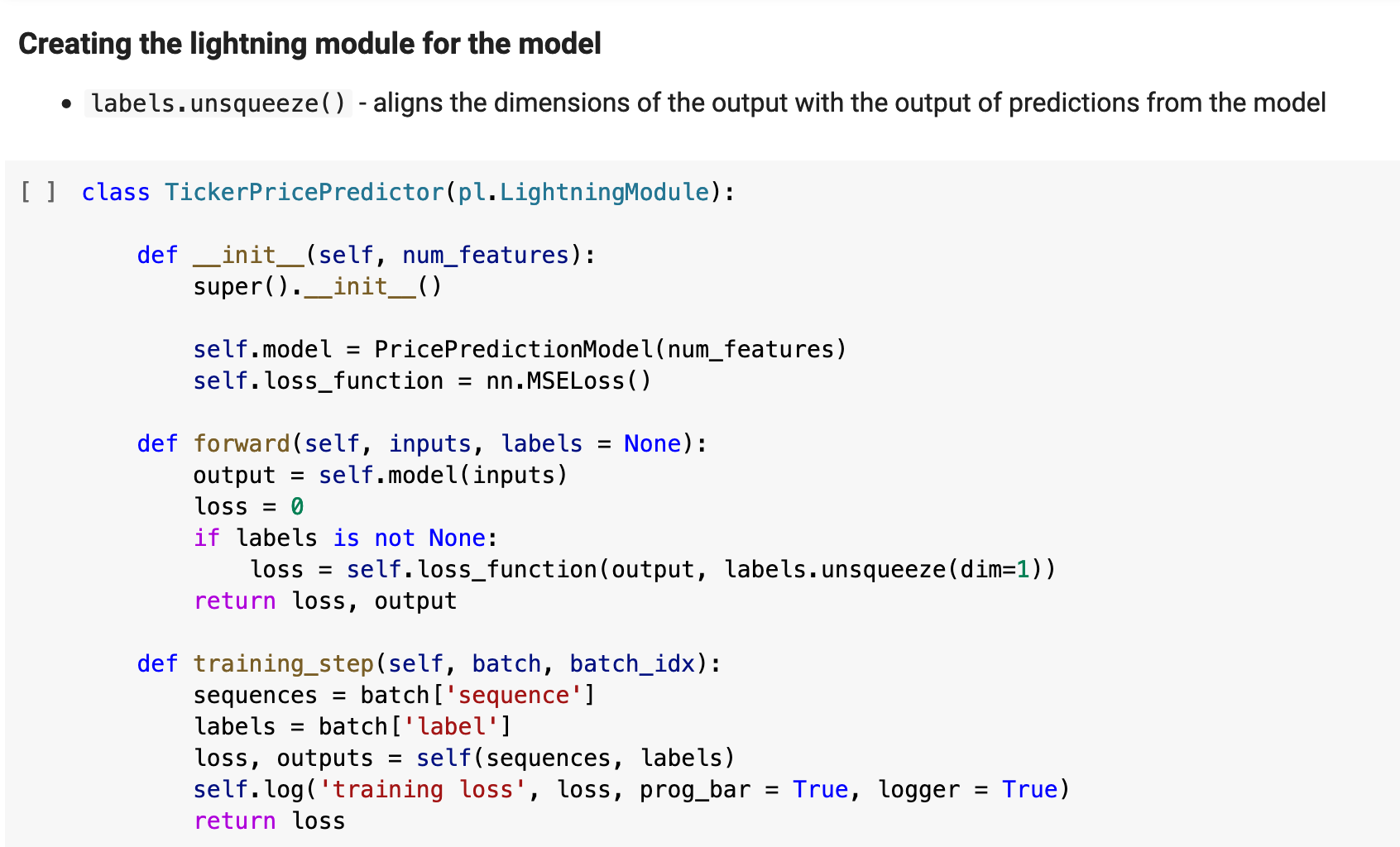
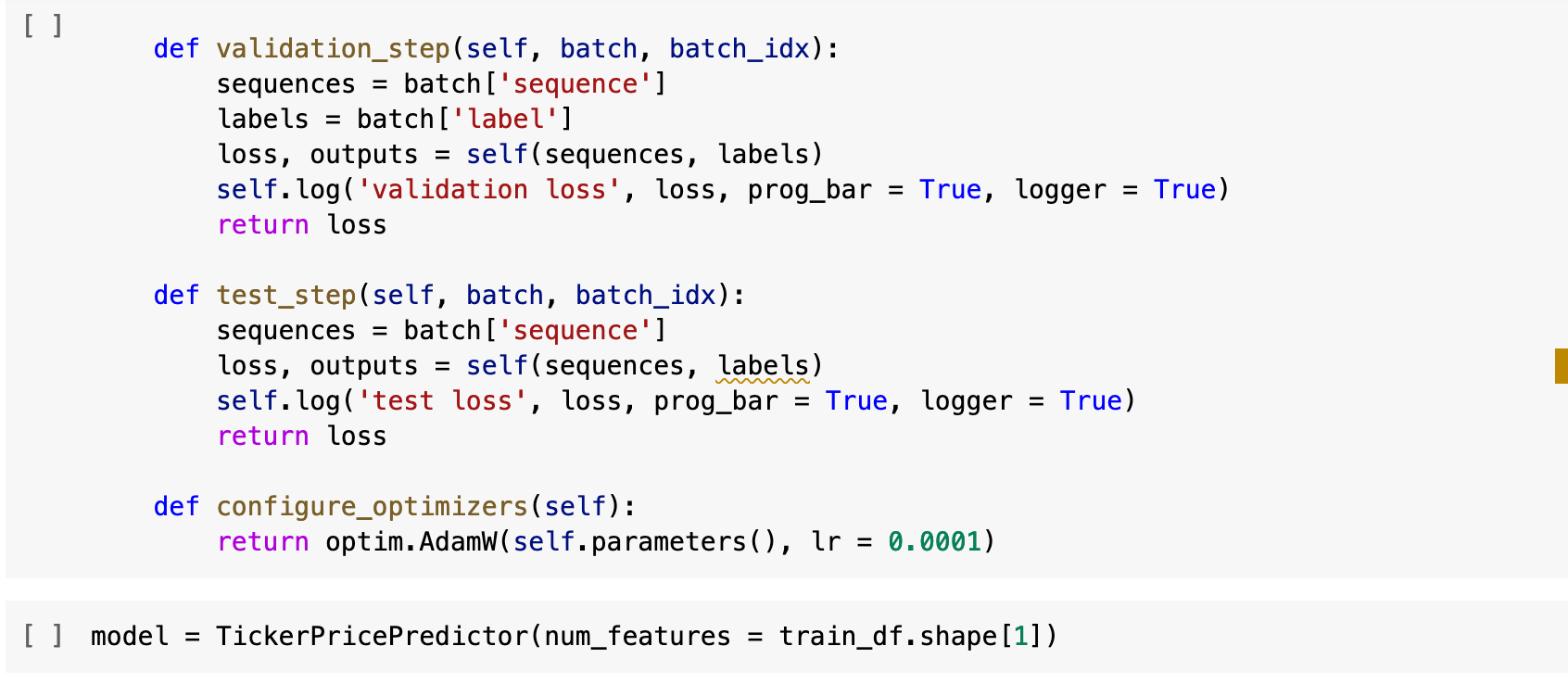
The following is the PyTorch Lightning module definition for the model, which will use the dataloaders defined in the class above in the training of the model. This defines each step along the way of training, as well as the logging of the entire training process.

8. Creating the Trainer and Training the Model

Before training, let's get one final look at the data we are passing in, just to be sure our dimensions all line up with our expectations. And they do!

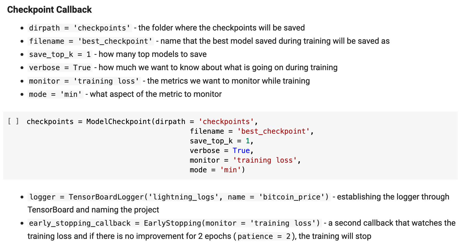
Here I am setting up the callbacks and monitoring for PyTorch Lightning. Note: Tensorboard logging caused a number of issues not only in my own environment, but also in Google Colab, so I decided not to incorporate it as a part of this project. I did, however, leave the notes concerning Tensorboard, for future reference. Below, you will find explanations of each aspect of this architecture.

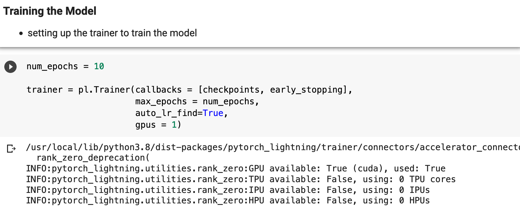
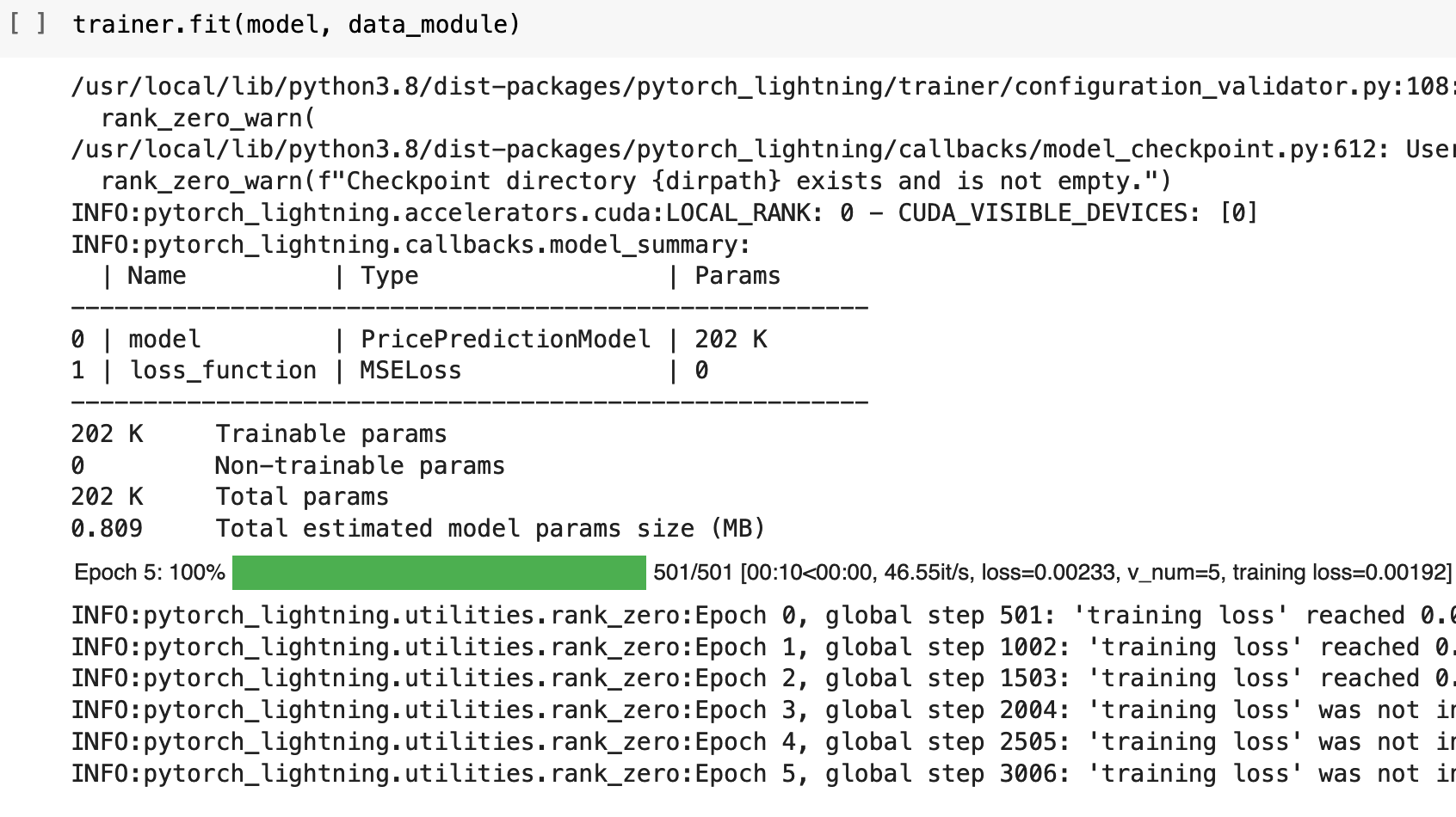
And now we get to define the trainer and train the model! I will train for 10 epochs, but as you will see, PyTorch Lightning catches me with early stopping and calls it quits early, since the model was no longer progressing.

9. The Results

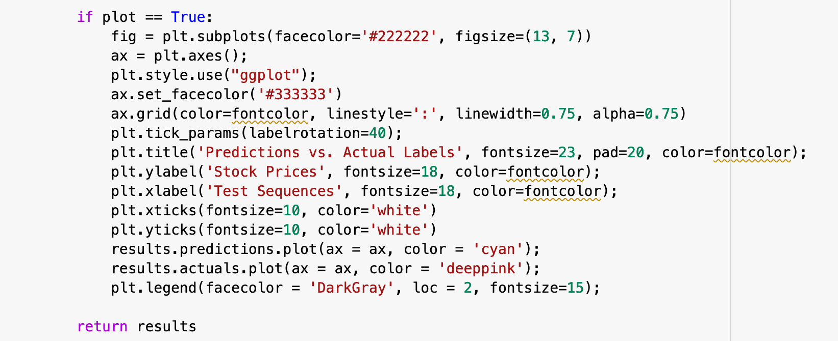
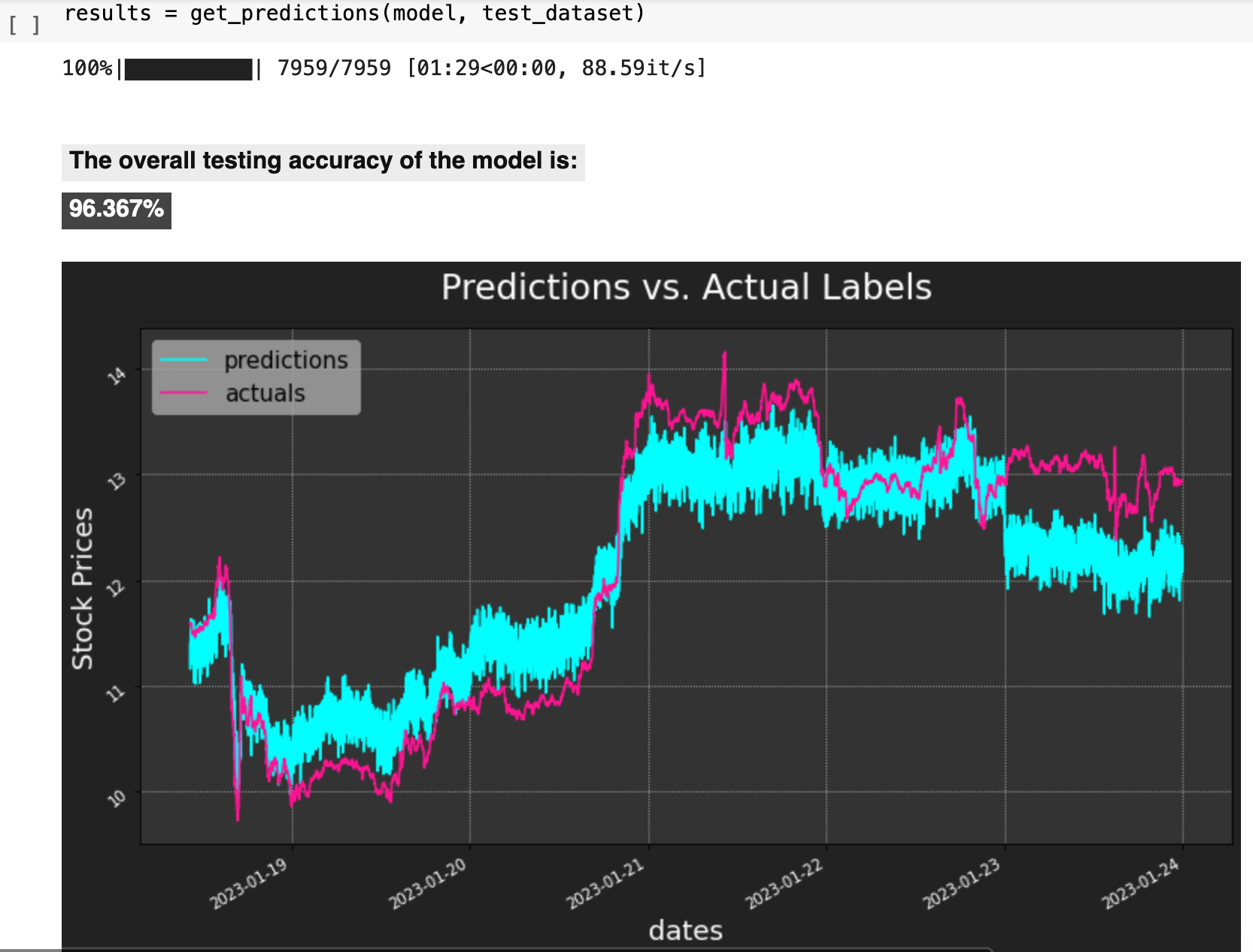
And now we can view the results of all this hard work! I wrote the following function to put together all of the important aspects of the results from testing. get_predictions() essentially passes the test data to the model, gets the predictions, compares the predictions for each record to the actual label for each record, computes the accuracy for each, as well as the overall average accuracy, and plots the predictions versus the actual labels.

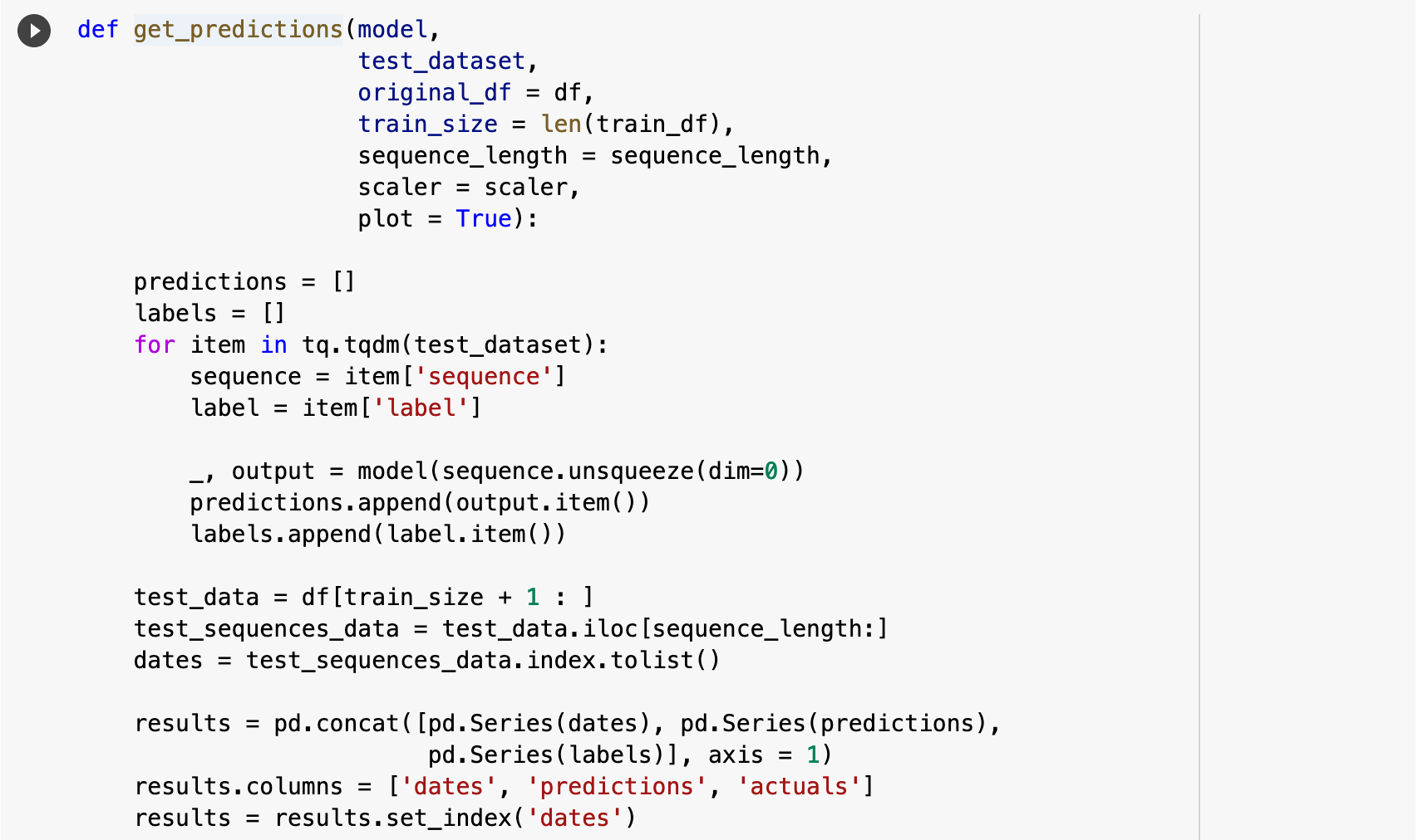
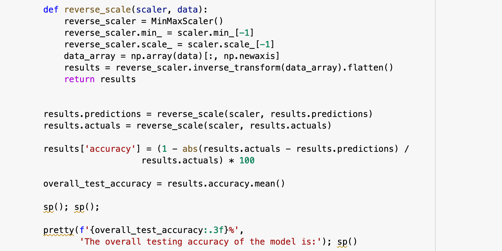
All of that for an overall testing accuracy of 96.367%.

So there you have it: a quick overview of ethereum price prediction with PyTorch, PyTorch Lightning, and an LSTM neural network model! I hope you enjoyed it and learned something new along the way.

May your features be many and your data be clean and complete! Happy data wrangling!