---

| Top | SciKit-Learn Way | SKTime Way | Multivariate | Panel Data | SKLearn & SKTime | Univariate Forecasting | Advanced Workflow | Forecasting with Exogeneous | Building a Forecaster | Time Series Classification | Time Series Regression |
SKTime
| Documentation | PyData Global 2021 | SKTime GitHub |

from helpers_new import * 
from sklearn.datasets import load_diabetes
import matplotlib as mpl
from tqdm.notebook import tqdm_notebook as tq
import time
%matplotlib inline
plt.style.use('dark_blue_greens.mplstyle')
css_styling()

---

| Top | SciKit-Learn Way | SKTime Way | Multivariate | Panel Data | SKLearn & SKTime | Univariate Forecasting | Advanced Workflow | Forecasting with Exogeneous | Building a Forecaster | Time Series Classification | Time Series Regression |
The SciKit-Learn Way

Diabetes Dataset (documentation)

Ten baseline variables, age, sex, body mass index, average blood pressure, and six blood serum measurements were obtained for each of n = 442 diabetes patients, as well as the response of interest, a quantitative measure of disease progression one year after baseline.

diabetes = load_diabetes()
input_data = diabetes['data']
target_data = diabetes['target']
input_df = pd.DataFrame(input_data, columns = diabetes['feature_names'])
target_series = pd.Series(target_data)

Inputs and Targets

• each input row is a different patient and their various data
  
• the target data is the disease progression

head_tail_vert(input_df, 5, 'diabetes: input_data')

diabetes: input_data: head(5)

	age	sex	bmi	bp	s1	s2	s3	s4	s5	s6
0	0.04	0.05	0.06	0.02	-0.04	-0.03	-0.04	-0.00	0.02	-0.02
1	-0.00	-0.04	-0.05	-0.03	-0.01	-0.02	0.07	-0.04	-0.07	-0.09
2	0.09	0.05	0.04	-0.01	-0.05	-0.03	-0.03	-0.00	0.00	-0.03
3	-0.09	-0.04	-0.01	-0.04	0.01	0.02	-0.04	0.03	0.02	-0.01
4	0.01	-0.04	-0.04	0.02	0.00	0.02	0.01	-0.00	-0.03	-0.05

diabetes: input_data: tail(5)

	age	sex	bmi	bp	s1	s2	s3	s4	s5	s6
437	0.04	0.05	0.02	0.06	-0.01	-0.00	-0.03	-0.00	0.03	0.01
438	-0.01	0.05	-0.02	-0.07	0.05	0.08	-0.03	0.03	-0.02	0.04
439	0.04	0.05	-0.02	0.02	-0.04	-0.01	-0.02	-0.01	-0.05	0.02
440	-0.05	-0.04	0.04	0.00	0.02	0.02	-0.03	0.03	0.04	-0.03
441	-0.05	-0.04	-0.07	-0.08	0.08	0.03	0.17	-0.04	-0.00	0.00

head_tail_horz(target_series, 5, "diabetes: target_data")

diabetes: target_data

head(5)

	0
0	151.00
1	75.00
2	141.00
3	206.00
4	135.00

   

tail(5)

	0
437	178.00
438	104.00
439	132.00
440	220.00
441	57.00

   

Initial Visualization

cols = list(input_df.columns)

def plot_feature(df, 
				 column, 
				 color = None,
				 title = None,
				 xlabel = None, 
				 ylabel = None):
	
	if color:
		color = color
	else:
		color = 'C0'
	
	cols = list(input_df.columns)
	fig, ax = plt.subplots(1)
	col = cols.index(column)
	ax.scatter(input_data[:,col], target_data, color = color)
	ax.set_title(f'{column} vs. {ylabel}')
	ax.set(
		xlabel = f'{xlabel}: {diabetes["feature_names"][col]}',
		ylabel = f'{ylabel}');
	

Visualization: age vs disease progression

plot_feature(input_data, 
			 'age', 
			 xlabel = 'blood serum measurement', 
			 ylabel = 'disease progression')

Visualization: bmi vs disease progression

plot_feature(input_data, 
			 'bmi', 
			 xlabel = 'blood serum measurement', 
			 ylabel = 'disease progression',
			 color = 'C1')

Visualization: bp vs disease progression

plot_feature(input_data, 
			 'bp', 
			 xlabel = 'blood serum measurement', 
			 ylabel = 'disease progression',
			 color = 'C2')

Workflow with SciKit-Learn

1. Model Specification
2. Fitting
3. Prediction
4. Evaluation

from sklearn.ensemble import RandomForestRegressor
from sklearn.metrics import mean_squared_error
from sklearn.model_selection import train_test_split

train_in, test_in, train_out, test_out = train_test_split(input_df, target_series)
pretty(f'train_in.shape: {train_in.shape}')
pretty(f'train_out.shape: {train_out.shape}')
pretty(f'test_in.shape: {test_in.shape}')
pretty(f'test_out.shape: {test_out.shape}')

train_in.shape: (331, 10)

train_out.shape: (331,)

test_in.shape: (111, 10)

test_out.shape: (111,)

Model

classifier = RandomForestRegressor()
classifier.fit(train_in, train_out)

RandomForestRegressor()

In a Jupyter environment, please rerun this cell to show the HTML representation or trust the notebook.
On GitHub, the HTML representation is unable to render, please try loading this page with nbviewer.org.

predictions = classifier.predict(test_in)

mean_squared_error(test_out, predictions)

3599.5111306306303

Modular Model Building & Pipelines with SciKit-Learn

• Pipelining and transformers
• Tuning
• Ensembling

from sklearn.neighbors import KNeighborsRegressor
from sklearn.pipeline import make_pipeline
from sklearn.preprocessing import StandardScaler

pipeline = make_pipeline(StandardScaler(), KNeighborsRegressor())
pipeline

Pipeline(steps=[('standardscaler', StandardScaler()),
                ('kneighborsregressor', KNeighborsRegressor())])

In a Jupyter environment, please rerun this cell to show the HTML representation or trust the notebook.
On GitHub, the HTML representation is unable to render, please try loading this page with nbviewer.org.

pipeline.fit(train_in, train_out)

Pipeline(steps=[('standardscaler', StandardScaler()),
                ('kneighborsregressor', KNeighborsRegressor())])

In a Jupyter environment, please rerun this cell to show the HTML representation or trust the notebook.
On GitHub, the HTML representation is unable to render, please try loading this page with nbviewer.org.

predictions = pipeline.predict(test_in)
mean_squared_error(test_out, predictions)

3670.1308108108105

Summary

• cross-selectional input data, without any assumed temporal dependency or ordering
• three learning tasks: cross-sectional classification, regression, clustering
• a common estimator API for each learning task
• estimator APIs mirror learning tasks

---

| Top | SciKit-Learn Way | SKTime Way | Multivariate | Panel Data | SKLearn & SKTime | Univariate Forecasting | Advanced Workflow | Forecasting with Exogeneous | Building a Forecaster | Time Series Classification | Time Series Regression |
The SKTime Way

• Check out tutorial from PyData Amsterdam 2020 on GitHub
• Simplest form of time series data is univariate, which has repeated observations of one variable or kind of measurement over time

Lynx Dataset (documentation)

The annual numbers of lynx trappings for 1821–1934 in Canada. This time-series records the number of skins of predators (lynx) that were collected over several years by the Hudson’s Bay Company. The dataset was taken from Brockwell & Davis (1991) and appears to be the series considered by Campbell & Walker (1977).

Dimensionality: univariate Series length: 114 Frequency: Yearly Number of cases: 1

This data shows aperiodic, cyclical patterns, as opposed to periodic, seasonal patterns.

from sktime.datasets import load_lynx
from sktime.utils.plotting import plot_series

lynx = load_lynx()
plot_series(lynx, title = 'Plotting a Univariate Time Series', colors = ['C4']);

---

| Top | SciKit-Learn Way | SKTime Way | Multivariate | Panel Data | SKLearn & SKTime | Univariate Forecasting | Advanced Workflow | Forecasting with Exogeneous | Building a Forecaster | Time Series Classification | Time Series Regression |
Multivariate Data

* Repeated observations over time from multiple related variables or kinds of measurement

Longley Dataset (documentation)

This mulitvariate time series dataset contains various US macroeconomic variables from 1947 to 1962 that are known to be highly collinear.

Dimensionality: multivariate, 6 Series length: 16 Frequency: Yearly Number of cases: 1

Variable description:

TOTEMP - Total employment GNPDEFL - Gross national product deflator GNP - Gross national product UNEMP - Number of unemployed ARMED - Size of armed forces POP - Population

from sktime.datasets import load_longley

targets, inputs = load_longley()

head_tail_horz(inputs, 5, 'Inputs')

Inputs

head(5)

	GNPDEFL	GNP	UNEMP	ARMED	POP
Period
1947	83.00	234,289.00	2,356.00	1,590.00	107,608.00
1948	88.50	259,426.00	2,325.00	1,456.00	108,632.00
1949	88.20	258,054.00	3,682.00	1,616.00	109,773.00
1950	89.50	284,599.00	3,351.00	1,650.00	110,929.00
1951	96.20	328,975.00	2,099.00	3,099.00	112,075.00

   

tail(5)

	GNPDEFL	GNP	UNEMP	ARMED	POP
Period
1958	110.80	444,546.00	4,681.00	2,637.00	121,950.00
1959	112.60	482,704.00	3,813.00	2,552.00	123,366.00
1960	114.20	502,601.00	3,931.00	2,514.00	125,368.00
1961	115.70	518,173.00	4,806.00	2,572.00	127,852.00
1962	116.90	554,894.00	4,007.00	2,827.00	130,081.00

   

head_tail_horz(targets, 5, 'Targets')

Targets

head(5)

	TOTEMP
Period
1947	60,323.00
1948	61,122.00
1949	60,171.00
1950	61,187.00
1951	63,221.00

   

tail(5)

	TOTEMP
Period
1958	66,513.00
1959	68,655.00
1960	69,564.00
1961	69,331.00
1962	70,551.00

   

Visualization: multiple input series

plot_series(targets, colors = ["C0"])
for idx, column in enumerate(inputs.columns[:2]):
	current = inputs[column]
	plot_series(current, colors = ["C" + str(idx+1)])

---

| Top | SciKit-Learn Way | SKTime Way | Multivariate | Panel Data | SKLearn & SKTime | Univariate Forecasting | Advanced Workflow | Forecasting with Exogeneous | Building a Forecaster | Time Series Classification | Time Series Regression |
Panel Data

• repeated observations over time on multiple independent experimental units from one or more related variables or kids of measurement

Arrowhead Dataset (documentation)

Dimensionality: univariate Series length: 251 Train cases: 36 Test cases: 175 Number of classes: 3

The arrowhead data consists of outlines of the images of arrowheads. The shapes of the projectile points are converted into a time series using the angle-based method. The classification of projectile points is an important topic in anthropology. The classes are based on shape distinctions such as the presence and location of a notch in the arrow. The problem in the repository is a length normalised version of that used in Ye09shapelets. The three classes are called “Avonlea”, “Clovis” and “Mix”.”

import matplotlib.pyplot as plt
from sktime.datasets import load_arrow_head
from sktime.datatypes import convert

inputs, targets = load_arrow_head(return_X_y = True)

head_tail_horz(inputs, 5, 'input data')

input data

head(5)

	dim_0
0	0 -1.96 1 -1.96 2 -1.96 3 -1.94 4 -1.90 ... 246 -1.84 247 -1.88 248 -1.91 249 -1.92 250 -1.91 Length: 251, dtype: float64
1	0 -1.77 1 -1.77 2 -1.78 3 -1.73 4 -1.70 ... 246 -1.64 247 -1.68 248 -1.73 249 -1.78 250 -1.79 Length: 251, dtype: float64
2	0 -1.87 1 -1.84 2 -1.84 3 -1.81 4 -1.76 ... 246 -1.83 247 -1.88 248 -1.86 249 -1.86 250 -1.85 Length: 251, dtype: float64
3	0 -2.07 1 -2.07 2 -2.04 3 -2.04 4 -1.96 ... 246 -1.95 247 -2.01 248 -2.03 249 -2.07 250 -2.08 Length: 251, dtype: float64
4	0 -1.75 1 -1.74 2 -1.72 3 -1.70 4 -1.68 ... 246 -1.72 247 -1.74 248 -1.74 249 -1.76 250 -1.76 Length: 251, dtype: float64

   

tail(5)

	dim_0
206	0 -1.63 1 -1.62 2 -1.63 3 -1.61 4 -1.57 ... 246 -1.57 247 -1.60 248 -1.62 249 -1.62 250 -1.62 Length: 251, dtype: float64
207	0 -1.66 1 -1.66 2 -1.63 3 -1.61 4 -1.59 ... 246 -1.68 247 -1.67 248 -1.67 249 -1.68 250 -1.68 Length: 251, dtype: float64
208	0 -1.60 1 -1.59 2 -1.58 3 -1.56 4 -1.53 ... 246 -1.58 247 -1.59 248 -1.60 249 -1.61 250 -1.61 Length: 251, dtype: float64
209	0 -1.74 1 -1.74 2 -1.73 3 -1.72 4 -1.70 ... 246 -1.64 247 -1.67 248 -1.70 249 -1.71 250 -1.73 Length: 251, dtype: float64
210	0 -1.63 1 -1.63 2 -1.62 3 -1.61 4 -1.58 ... 246 -1.51 247 -1.55 248 -1.58 249 -1.60 250 -1.62 Length: 251, dtype: float64

   

head_tail_horz(targets, 5, 'target data')

target data

head(5)

	0
0	0
1	1
2	2
3	0
4	1

   

tail(5)

	0
206	2
207	2
208	2
209	2
210	2

   

pretty(inputs.shape, 'inputs.shape before conversion')

inputs.shape before conversion
(211, 1)

inputs = convert(inputs, from_type = 'nested_univ', to_type = 'numpy3D')

pretty(inputs.shape, 'inputs.shape after conversion')

inputs.shape after conversion
(211, 1, 251)

labels, counts = np.unique(targets, return_counts = True)

Visualization: multiple input samples

fig, ax = plt.subplots(1, figsize = plt.figaspect(0.25))
for label in labels: 
	ax.plot(inputs[targets == label, 0, :][0], label = f'class {label}');
ax.set(ylabel = 'Scaled Distance from Midpoint', xlabel = 'Index');
ax.set_title('Panel Data: Each line represents a different, independent sample');

labels, counts = np.unique(targets, return_counts = True)
fig, ax = plt.subplots(1, figsize = plt.figaspect(0.25))
for label in labels: 
	for idx in range(3):
		ax.plot(inputs[targets == label, 0, :][idx], label = f'class {label}');
ax.set(ylabel = 'Scaled Distance from Midpoint', xlabel = 'Index');
ax.set_title('Panel Data: Each line represents a different, independent sample');

---

| Top | SciKit-Learn Way | SKTime Way | Multivariate | Panel Data | SKLearn & SKTime | Univariate Forecasting | Advanced Workflow | Forecasting with Exogeneous | Building a Forecaster | Time Series Classification | Time Series Regression |
SKLearn + SKTime: Multiple Learning Tasks

• Forecasting (different variations) - predicting future values for a time serie
• Time Series Classification - classifying a time series
• Time Series Annotation (e.g. outlier detection) - assigning labels or annotation to time points in a time series
• Time Series Clustering - identifying and grouping similar time series

Reduction: From one learning task to another

**Overview**

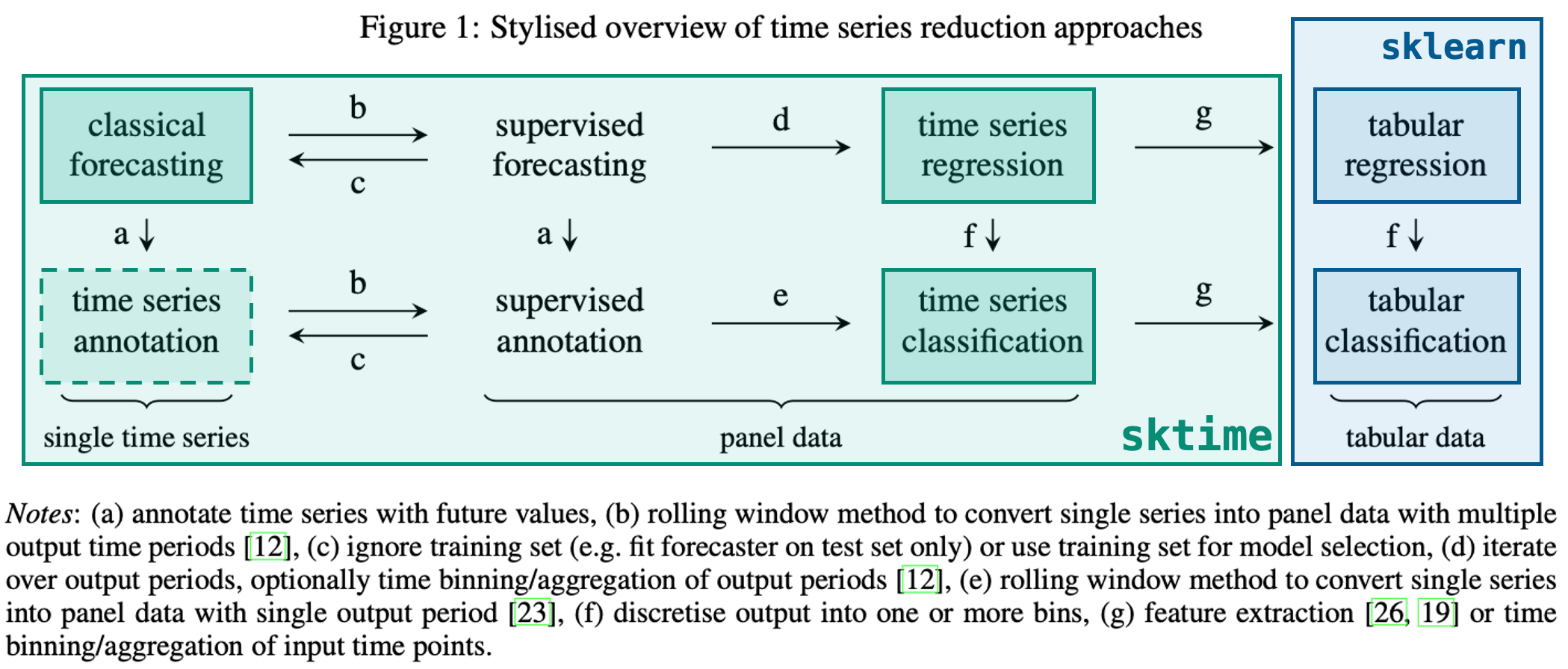
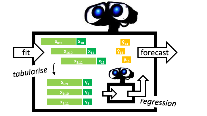
**Example: From forecasting to regression**

Creating a unified framework

• time-series input data
• multiple learning tasks: forecasting, time series classification and more
• a common estimator API for each learning task
• estimator APIs mirror learning tasks

What's a framework?

Check out our glossary of common terms:

A collection of related and reusable software design templates that practitioners can copy and fill in. Frameworks emphasize design reuse. They capture common software design decisions within a given application domain and distill them into reusable design templates. This reduces the design decision they must take, allowing them to focus on application specifics. Not only can practitioners write software faster as a result, but applications will have a similar structure. Frameworks often offer additional functionality like toolboxes. Compare with toolbox and application.

Check out our extension templates!

---

| Top | SciKit-Learn Way | SKTime Way | Multivariate | Panel Data | SKLearn & SKTime | Univariate Forecasting | Advanced Workflow | Forecasting with Exogeneous | Building a Forecaster | Time Series Classification | Time Series Regression |
Univariate Forecasting

• Univariate
• Univariate with exogenous variables
• Multivariate

---

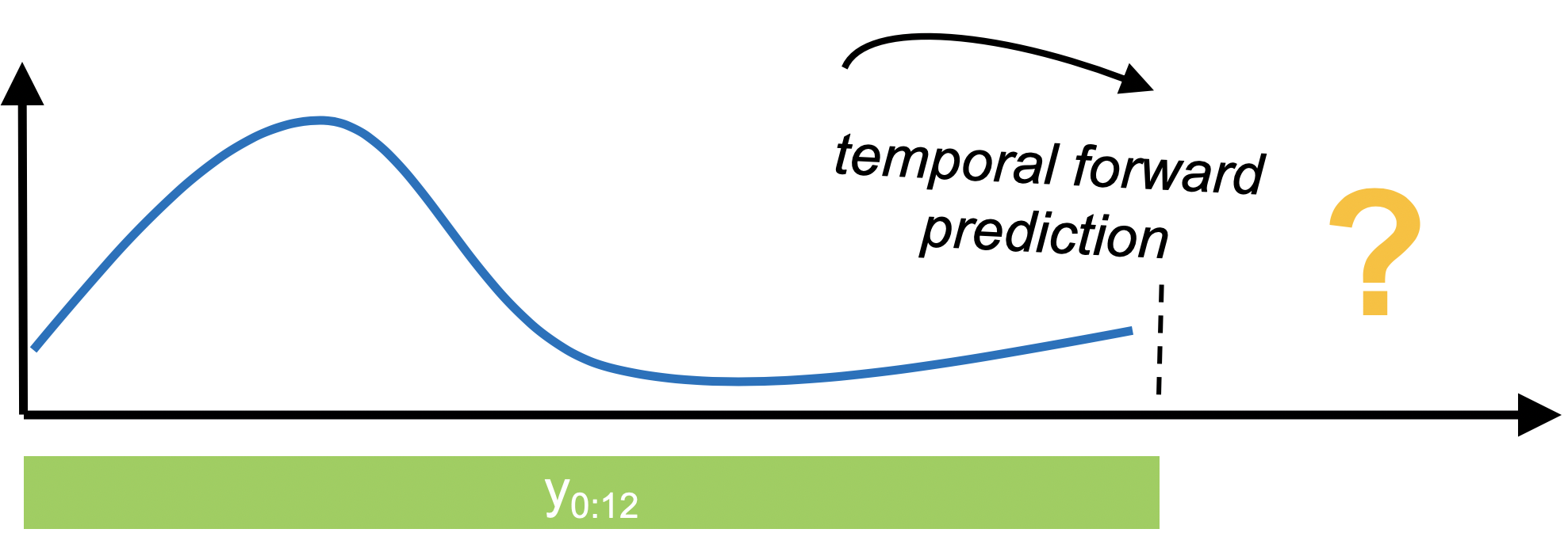
Univariate forecasting

In forecasting, we're interested in using past data to make temporal forward predictions. sktime provides common statistical forecasting algorithms and tools for building composite machine learning models.

The basic workflow

1. Specify data
2. Specify task
3. Specify model
4. Fit
5. Predict

from warnings import simplefilter
simplefilter(action="ignore", category=RuntimeWarning)

from sktime.datasets import load_shampoo_sales
from sktime.utils.plotting import plot_series

Data Specification

Shampoo Sales Dataset (documentation)

This dataset describes the monthly number of sales of shampoo over a 3 year period. The units are a sales count.

Dimensionality: univariate Series length: 36 Frequency: Monthly Number of cases: 1

shampoo_data = load_shampoo_sales()
plot_series(shampoo_data, title = "Shampoo Sales Time Series", 
		   colors = ['C4']);

Task specification

Next we will define a **forecasting task**

• We will try to predict the last 6 months of data, using the previous data as training data. Each point in the series represents a month, so we should hold out the last 6 points as test data, and use 6-step ahead forecasting horizon to evaluate forecasting performance.
• We will use the MAPE (mean absolute percentage error) to quantify the accuracy of our forecasts. A lower MAPE means higher accuracy.

The Forecasting Horizon

When we want to generate forecasts, we need to specify the forecasting horizon and pass that to our forecasting algorithm. We can specify the forecasting horizon as a numpy array of the steps ahead relative to the end of the training series:

• ForcastingHorizon()
• is_relative = False - to specify exact dates. True (default) means that each time point will be relative to the last time point in the data

Init signature:
ForecastingHorizon(
    values: Union[int, list, numpy.ndarray, pandas.core.indexes.base.Index] = None,
    is_relative: bool = None,
    freq=None,
)
Docstring:     
Forecasting horizon.

Parameters
----------
values : pd.Index, pd.TimedeltaIndex, np.array, list, pd.Timedelta, or int
    Values of forecasting horizon
is_relative : bool, optional (default=None)
    - If True, a relative ForecastingHorizon is created:
            values are relative to end of training series.
    - If False, an absolute ForecastingHorizon is created:
            values are absolute.
    - if None, the flag is determined automatically:
        relative, if values are of supported relative index type
        absolute, if not relative and values of supported absolute index type
freq : str, pd.Index, pandas offset, or sktime forecaster, optional (default=None)
    object carrying frequency information on values
    ignored unless values is without inferrable freq

import numpy as np

horizon = np.arange(6) + 1

pretty(horizon, 'Forecasting Horizon: np.arange(6) + 1 -> Relative')

Forecasting Horizon: np.arange(6) + 1 -> Relative
[1, 2, 3, 4, 5, 6]

import pandas as pd
from sktime.forecasting.base import ForecastingHorizon

horizon = ForecastingHorizon(
    pd.period_range("1993-07", periods=6, freq="M"), is_relative=False
)

pretty(horizon, 'Forecasting Horizon: pd.period_range("1993-07", periods=6, freq="M) -> Absolute')

Forecasting Horizon: pd.period_range("1993-07", periods=6, freq="M) -> Absolute
ForecastingHorizon(['1993-07', '1993-08', '1993-09', '1993-10', '1993-11', '1993-12'], dtype='period[M]', is_relative=False)

Converting between absolute and relative forecast horizons

to_relative() - cutoff allows you to determin when/where to convert to relative from absolute

Signature: ForecastingHorizon.to_relative(self, cutoff=None) Docstring: Return forecasting horizon values relative to a cutoff.

Parameters

cutoff : pd.Period, pd.Timestamp, int, or pd.Index, optional (default=None)
    Cutoff value required to convert a relative forecasting
    horizon to an absolute one (and vice versa).
    If pd.Index, last/latest value is considered the cutoff

Returns

fh : ForecastingHorizon
    Relative representation of forecasting horizon.

cutoff = pd.Period("1993-06", freq="M")
pretty(horizon.to_relative(cutoff), 'cutoff = pd.Period("1993-06", freq="M") | horizon.to_relative(cutoff)')

cutoff = pd.Period("1993-06", freq="M") | horizon.to_relative(cutoff)
ForecastingHorizon([1, 2, 3, 4, 5, 6], dtype='int64', is_relative=True)

Splitting: temporal_train_test_split()

Signature:
temporal_train_test_split(
    y: Union[pandas.core.series.Series, pandas.core.frame.DataFrame, numpy.ndarray, pandas.core.indexes.base.Index],
    X: Optional[pandas.core.frame.DataFrame] = None,
    test_size: Union[int, float, NoneType] = None,
    train_size: Union[int, float, NoneType] = None,
    fh: Union[int, list, numpy.ndarray, pandas.core.indexes.base.Index, sktime.forecasting.base._fh.ForecastingHorizon, NoneType] = None,
) -> Union[Tuple[pandas.core.series.Series, pandas.core.series.Series], Tuple[pandas.core.series.Series, pandas.core.series.Series, pandas.core.frame.DataFrame, pandas.core.frame.DataFrame]]
Docstring:
Split arrays or matrices into sequential train and test subsets.

Creates train/test splits over endogenous arrays an optional exogenous
arrays.

This is a wrapper of scikit-learn's ``train_test_split`` that
does not shuffle the data.

Parameters
----------
y : pd.Series
    Target series
X : pd.DataFrame, optional (default=None)
    Exogenous data
test_size : float, int or None, optional (default=None)
    If float, should be between 0.0 and 1.0 and represent the proportion
    of the dataset to include in the test split. If int, represents the
    relative number of test samples. If None, the value is set to the
    complement of the train size. If ``train_size`` is also None, it will
    be set to 0.25.
train_size : float, int, or None, (default=None)
    If float, should be between 0.0 and 1.0 and represent the
    proportion of the dataset to include in the train split. If
    int, represents the relative number of train samples. If None,
    the value is automatically set to the complement of the test size.
fh : ForecastingHorizon

Returns
-------
splitting : tuple, length=2 * len(arrays)
    List containing train-test split of `y` and `X` if given.

from sktime.forecasting.model_selection import temporal_train_test_split

train_targets, test_targets = temporal_train_test_split(shampoo_data, 
														   fh=horizon)

Visualization: forecast horizon for train-test split

plot_series(train_targets, 
			test_targets, 
			labels=["train_targets", "test_targets"],
		    colors = ['C4', 'C0'],
		    title = 'Using Forecast Horizon to Train-Test Split');

Model Specification: NaiveForecaster()

**NaiveForecaster** is a forecaster that makes forecasts using simple strategies. Two out of three strategies are robust against NaNs. The NaiveForecaster can also be used for multivariate data and it then applies internally the ColumnEnsembleForecaster, so each column is forecasted with the same strategy.

Internally, this forecaster does the following:

• obtains the so-called "last window", a 1D array that denotes the most recent time window that the forecaster is allowed to use
• reshapes the last window into a 2D array according to the given seasonal periodicity (prepended with NaN values to make it fit);
• make a prediction for each column, using the given strategy:
  • "last": last non-NaN row
  • "mean": np.nanmean over rows
• tile the predictions using the seasonal periodicity

To compute prediction quantiles, we first estimate the standard error of prediction residuals under the assumption of uncorrelated residuals. The forecast variance is then computed by multiplying the residual variance by a constant. This constant is a small-sample bias adjustment and each method (mean, last, drift) have different formulas for computing the constant. These formulas can be found in the Forecasting: Principles and Practice textbook (Table 5.2) [1]_. Lastly, under the assumption that residuals follow a normal distribution, we use the forecast variance and z-scores of a normal distribution to estimate the prediction quantiles.

Parameters
----------
strategy : {"last", "mean", "drift"}, default="last"
    Strategy used to make forecasts:

    * "last":   (robust against NaN values)
                forecast the last value in the
                training series when sp is 1.
                When sp is not 1,
                last value of each season
                in the last window will be
                forecasted for each season.
    * "mean":   (robust against NaN values)
                forecast the mean of last window
                of training series when sp is 1.
                When sp is not 1, mean of all values
                in a season from last window will be
                forecasted for each season.
    * "drift":  (not robust against NaN values)
                forecast by fitting a line between the
                first and last point of the window and
                extrapolating it into the future.

sp : int, or None, default=1
    Seasonal periodicity to use in the seasonal forecasting. None=1.

window_length : int or None, default=None
    Window length to use in the `mean` strategy. If None, entire training
        series will be used.

from sktime.forecasting.naive import NaiveForecaster

forecaster = NaiveForecaster(strategy="drift", window_length=10)

Model Fitting: NaiveForecaster.fit()

• y - always required
• X - exogenous data

  In an economic model, an exogenous variable is one whose measure is determined outside the model and is imposed on the model, and an exogenous change is a change in an exogenous variable

• fh - can pass forecast horizon either in fitting or predicting

Signature: forecaster.fit(y, X=None, fh=None)
Docstring:
Fit forecaster to training data.

State change:
    Changes state to "fitted".

Writes to self:
    Sets self._is_fitted flag to True.
    Writes self._y and self._X with `y` and `X`, respectively.
    Sets self.cutoff and self._cutoff to last index seen in `y`.
    Sets fitted model attributes ending in "_".
    Stores fh to self.fh if fh is passed.

Parameters
----------
y : time series in sktime compatible data container format
        Time series to which to fit the forecaster.
    y can be in one of the following formats:
    Series scitype: pd.Series, pd.DataFrame, or np.ndarray (1D or 2D)
        for vanilla forecasting, one time series
    Panel scitype: pd.DataFrame with 2-level row MultiIndex,
        3D np.ndarray, list of Series pd.DataFrame, or nested pd.DataFrame
        for global or panel forecasting
    Hierarchical scitype: pd.DataFrame with 3 or more level row MultiIndex
        for hierarchical forecasting
    Number of columns admissible depend on the "scitype:y" tag:
        if self.get_tag("scitype:y")=="univariate":
            y must have a single column/variable
        if self.get_tag("scitype:y")=="multivariate":
            y must have 2 or more columns
        if self.get_tag("scitype:y")=="both": no restrictions on columns apply
    For further details:
        on usage, see forecasting tutorial examples/01_forecasting.ipynb
        on specification of formats, examples/AA_datatypes_and_datasets.ipynb
fh : int, list, np.array or ForecastingHorizon, optional (default=None)
    The forecasting horizon encoding the time stamps to forecast at.
    if self.get_tag("requires-fh-in-fit"), must be passed, not optional
X : time series in sktime compatible format, optional (default=None)
        Exogeneous time series to fit to
    Should be of same scitype (Series, Panel, or Hierarchical) as y
    if self.get_tag("X-y-must-have-same-index"), X.index must contain y.index
    there are no restrictions on number of columns (unlike for y)

forecaster.fit(train_targets)

NaiveForecaster(strategy='drift', window_length=10)

In a Jupyter environment, please rerun this cell to show the HTML representation or trust the notebook.
On GitHub, the HTML representation is unable to render, please try loading this page with nbviewer.org.

Predicting: NaiveForecaster.predict()

Signature: NaiveForecaster.predict(self, fh=None, X=None)
Docstring:
Forecast time series at future horizon.

State required:
    Requires state to be "fitted".

Accesses in self:
    Fitted model attributes ending in "_".
    self.cutoff, self._is_fitted

Writes to self:
    Stores fh to self.fh if fh is passed and has not been passed previously.

Parameters
----------
fh : int, list, np.array or ForecastingHorizon, optional (default=None)
    The forecasting horizon encoding the time stamps to forecast at.
    if has not been passed in fit, must be passed, not optional
X : time series in sktime compatible format, optional (default=None)
        Exogeneous time series to fit to
    Should be of same scitype (Series, Panel, or Hierarchical) as y in fit
    if self.get_tag("X-y-must-have-same-index"), X.index must contain fh.index
    there are no restrictions on number of columns (unlike for y)

Returns
-------
y_pred : time series in sktime compatible data container format
    Point forecasts at fh, with same index as fh
    y_pred has same type as the y that has been passed most recently:
        Series, Panel, Hierarchical scitype, same format (see above)

predictions = forecaster.predict(horizon)

plot_series(train_targets, 
			test_targets, 
			predictions,
			labels=['train_targets', 'test_targets', 'predictions'],
		    colors = ['C4', 'C0', 'C3'],
		    title = 'Linear Strategy Prediction');

Evaluation: mean_absolute_percentage_error()

from sktime.performance_metrics.forecasting import \
    mean_absolute_percentage_error

mean_absolute_percentage_error(test_targets, predictions, symmetric=False)

0.16469764622516225

Another Example: AutoARIMA

• using AutoARIMA() rather than NaiveForecaster()

from sktime.forecasting.arima import AutoARIMA

data = load_shampoo_sales()
training, testing = temporal_train_test_split(data, fh=horizon)
forecaster = AutoARIMA(sp=12, suppress_warnings=True)

forecaster.fit(training)

AutoARIMA(sp=12, suppress_warnings=True)

In a Jupyter environment, please rerun this cell to show the HTML representation or trust the notebook.
On GitHub, the HTML representation is unable to render, please try loading this page with nbviewer.org.

predictions = forecaster.predict(horizon)

plot_series(training, testing, predictions, 
			labels=["y_train", "y_test", "y_pred"],
		   colors = ['C4', 'C0', 'C3'],
		   title = 'Example: using AutoARIMA as a Model');

Summary of basic workflow

• single, fixed cutoff point at which we generate predictions
• common interface for forecasters

Forecasters in sktime

Check out our online estimator overview at: https://www.sktime.org/en/stable/estimator_overview.html

**all_estimators()**

Signature:
all_estimators(
    estimator_types=None,
    filter_tags=None,
    exclude_estimators=None,
    return_names=True,
    as_dataframe=False,
    return_tags=None,
    suppress_import_stdout=True,
)
Docstring:
Get a list of all estimators from sktime.

This function crawls the module and gets all classes that inherit
from sktime's and sklearn's base classes.

Not included are: the base classes themselves, classes defined in test
modules.

from sktime.registry import all_estimators

estimators = all_estimators("forecaster", as_dataframe=True)
head_tail_horz(estimators.name, 5, 'Forecaster Estimators (some options)')

Forecaster Estimators (some options)

head(5)

	name
0	ARDL
1	ARIMA
2	AutoARIMA
3	AutoETS
4	AutoEnsembleForecaster

   

tail(5)

	name
48	UpdateEvery
49	UpdateRefitsEvery
50	VAR
51	VARMAX
52	VECM

   

missing_data_estimators = all_estimators("forecaster", 
									   filter_tags = {"handles-missing-data": True}, 
									   as_dataframe=True)

head_tail_horz(missing_data_estimators.name.sample(10), 5, 
			   'Forecaster Estimators (using filters)')

Forecaster Estimators (using filters)

head(5)

	name
6	DirectTimeSeriesRegressionForecaster
17	TransformedTargetForecaster
9	ForecastingPipeline
12	NaiveForecaster
11	MultioutputTimeSeriesRegressionForecaster

   

tail(5)

	name
10	MultioutputTabularRegressionForecaster
4	DirRecTimeSeriesRegressionForecaster
16	StackingForecaster
0	ARIMA
8	ForecastByLevel

   

But can I not just use scikit-learn?

In principle, yes, but many pitfalls ...

See our previous tutorial from the PyData Amsterdam 2020 for more details: https://github.com/sktime/sktime-tutorial-pydata-amsterdam-2020

Better: Use scikit-learn with sktime!

sktime provides a meta-estimator for this approach, which is:

• modular and compatible with scikit-learn, so that we can easily apply any scikit-learn regressor to solve our forecasting problem,
• parametric and tuneable, allowing us to tune hyper-parameters like the window length or strategy to generate forecasts
• adaptive, in the sense that it adapts the scikit-learn's estimator interface to that of a forecaster, making sure that we can tune and properly evaluate our model

Using a Scikit-Learn Model

Airline Passenger Dataset (documentation)

The classic Box & Jenkins airline data. Monthly totals of international airline passengers, 1949 to 1960.

Dimensionality: univariate Series length: 144 Frequency: Monthly Number of cases: 1

This data shows an increasing trend, non-constant (increasing) variance and periodic, seasonal patterns.

Visualization: airline passenger dataset input

from sktime.datasets import load_airline
from sktime.utils.plotting import plot_series

targets = load_airline()
plot_series(targets, colors = ['C6'], title = 'Airline Passenger Dataset');

train_targets, test_targets = temporal_train_test_split(targets, test_size=12)
horizon = ForecastingHorizon(test_targets.index, is_relative=False)

**`forecasting.compose.make_reduction()`**

Signature:
make_reduction(
    estimator,
    strategy='recursive',
    window_length=10,
    scitype='infer',
    transformers=None,
    pooling='local',
    windows_identical=True,
)
Docstring:
Make forecaster based on reduction to tabular or time-series regression.

During fitting, a sliding-window approach is used to first transform the
time series into tabular or panel data, which is then used to fit a tabular or
time-series regression estimator. During prediction, the last available data is
used as input to the fitted regression estimator to generate forecasts.

Parameters
----------
estimator : an estimator instance
    Either a tabular regressor from scikit-learn or a time series regressor from
    sktime.
strategy : str, optional (default="recursive")
    The strategy to generate forecasts. Must be one of "direct", "recursive" or
    "multioutput".
window_length : int, optional (default=10)
    Window length used in sliding window transformation.
scitype : str, optional (default="infer")
    Legacy argument for downwards compatibility, should not be used.
    `make_reduction` will automatically infer the correct type of `estimator`.
    This internal inference can be force-overridden by the `scitype` argument.
    Must be one of "infer", "tabular-regressor" or "time-series-regressor".
    If the scitype cannot be inferred, this is a bug and should be reported.
transformers: list of transformers (default = None)
    A suitable list of transformers that allows for using an en-bloc approach with
    make_reduction. This means that instead of using the raw past observations of
    y across the window length, suitable features will be generated directly from
    the past raw observations. Currently only supports WindowSummarizer (or a list
    of WindowSummarizers) to generate features e.g. the mean of the past 7
    observations. Currently only works for RecursiveTimeSeriesRegressionForecaster.
pooling: str {"local", "global"}, optional
    Specifies whether separate models will be fit at the level of each instance
    (local) of if you wish to fit a single model to all instances ("global").
    Currently only works for RecursiveTimeSeriesRegressionForecaster.
windows_identical: bool, (default = True)
    Direct forecasting only.
    Specifies whether all direct models use the same X windows from y (True: Number
    of windows = total observations + 1 - window_length - maximum forecasting
    horizon) or a different number of X windows depending on the forecasting horizon
    (False: Number of windows = total observations + 1 - window_length
    - forecasting horizon). See pictionary below for more information.

Visualization: SKLearn's KNeighbors with recursive strategy

from sklearn.neighbors import KNeighborsRegressor
from sktime.forecasting.compose import make_reduction

regressor = KNeighborsRegressor(n_neighbors=2)
forecaster = make_reduction(regressor, strategy="recursive", window_length=15)
forecaster.fit(train_targets, fh=horizon)
predictions = forecaster.predict()
plot_series(train_targets, test_targets, predictions, 
			labels=["train_targets", "test_targets", "predictions"],
		   colors = ['C0', 'C1', 'C2'],
		   title = 'KNeighborsRegressor | strategy = "recursive"');

Visualization: SKLearn's KNeighbors with multioutput strategy

regressor = KNeighborsRegressor(n_neighbors=1)
forecaster = make_reduction(regressor, strategy="multioutput", window_length=7)
forecaster.fit(train_targets, fh=horizon)
predictions = forecaster.predict()
plot_series(train_targets, test_targets, predictions, 
			labels=["train_targets", "test_targets", "predictions"],
		   colors = ['C0', 'C1', 'C2'],
		   title = 'KNeighborsRegressor | strategy = "multioutput"');

---

| Top | SciKit-Learn Way | SKTime Way | Multivariate | Panel Data | SKLearn & SKTime | Univariate Forecasting | Advanced Workflow | Forecasting with Exogeneous | Building a Forecaster | Time Series Classification | Time Series Regression |
More Advanced workflow

1. Specify data
2. Specify task
3. Specify model
4. Fit
5. Predict
6. Observe new data
7. Update using new data
8. Repeat steps 5-7 as often as required

Data specification

from sktime.forecasting.ets import AutoETS

data = load_airline()
plot_series(data, colors = ['C6'], title = 'Airline Data');

Task specification

# specifying the forecasting horizon: one year ahead, all months
# 12 steps ahead

horizon = np.arange(1, 13)
pretty(horizon, 'Forecast Horizon  |  np.arange(1, 13)')

Forecast Horizon | np.arange(1, 13)
[1, 2, 3, 4, 5, 6, 7, 8, 9, 10, 11, 12]

train_data = data.loc[:"1957-08"]
observed_data = train_data.copy()
observed_data.tail()

1957-04   348.00
1957-05   355.00
1957-06   422.00
1957-07   465.00
1957-08   467.00
Freq: M, Name: Number of airline passengers, dtype: float64

Model specification

forecaster = AutoETS(auto=True, sp=12, n_jobs=-1)

Fitting

forecaster.fit(train_data)

AutoETS(auto=True, n_jobs=-1, sp=12)

In a Jupyter environment, please rerun this cell to show the HTML representation or trust the notebook.
On GitHub, the HTML representation is unable to render, please try loading this page with nbviewer.org.

Prediction

predictions = forecaster.predict(horizon)
plot_series(observed_data, predictions, colors = ['C2', 'C6'], 
		   title = 'Predictions with AutoETS');

predictions

1957-09   413.46
1957-10   360.57
1957-11   314.50
1957-12   358.25
1958-01   363.38
1958-02   363.45
1958-03   417.74
1958-04   402.20
1958-05   398.85
1958-06   451.96
1958-07   498.86
1958-08   494.80
Freq: M, dtype: float64

Observe New Data

oberved_data = data.loc[:"1957-09"]
new_data = data.loc[["1957-09"]]
new_data

1957-09   404.00
Freq: M, Name: Number of airline passengers, dtype: float64

Update

forecaster.update(new_data)

/Users/evancarr/opt/anaconda3/envs/time_series_projects/lib/python3.10/site-packages/sktime/forecasting/base/_base.py:1881: UserWarning: NotImplementedWarning: AutoETS does not have a custom `update` method implemented. AutoETS will be refit each time `update` is called with update_params=True. To refit less often, use the wrappers in the forecasting.stream module, e.g., UpdateEvery.
  warn(

AutoETS(auto=True, n_jobs=-1, sp=12)

In a Jupyter environment, please rerun this cell to show the HTML representation or trust the notebook.
On GitHub, the HTML representation is unable to render, please try loading this page with nbviewer.org.

Predict again

predictions = forecaster.predict(horizon)
plot_series(observed_data, predictions,
		   colors = ['C3', 'C4'],
		   title = 'Updated Model Predictions');

predictions

1957-10   354.74
1957-11   309.49
1957-12   352.61
1958-01   357.73
1958-02   357.87
1958-03   411.40
1958-04   396.16
1958-05   392.94
1958-06   445.34
1958-07   491.65
1958-08   487.74
1958-09   432.52
Freq: M, dtype: float64

Understanding update()

• in order to update without updating the model's weights, specify update_params = False. (True by default)

forecaster.update?

Signature: forecaster.update(y, X=None, update_params=True)
Docstring:
Update cutoff value and, optionally, fitted parameters.

If no estimator-specific update method has been implemented,
default fall-back is as follows:
    update_params=True: fitting to all observed data so far
    update_params=False: updates cutoff and remembers data only

State required:
    Requires state to be "fitted".

Accesses in self:
    Fitted model attributes ending in "_".
    Pointers to seen data, self._y and self.X
    self.cutoff, self._is_fitted
    If update_params=True, model attributes ending in "_".

Writes to self:
    Update self._y and self._X with `y` and `X`, by appending rows.
    Updates self.cutoff and self._cutoff to last index seen in `y`.
    If update_params=True,
        updates fitted model attributes ending in "_".

Parameters
----------
y : time series in sktime compatible data container format
        Time series to which to fit the forecaster in the update.
    y can be in one of the following formats, must be same scitype as in fit:
    Series scitype: pd.Series, pd.DataFrame, or np.ndarray (1D or 2D)
        for vanilla forecasting, one time series
    Panel scitype: pd.DataFrame with 2-level row MultiIndex,
        3D np.ndarray, list of Series pd.DataFrame, or nested pd.DataFrame
        for global or panel forecasting
    Hierarchical scitype: pd.DataFrame with 3 or more level row MultiIndex
        for hierarchical forecasting
    Number of columns admissible depend on the "scitype:y" tag:
        if self.get_tag("scitype:y")=="univariate":
            y must have a single column/variable
        if self.get_tag("scitype:y")=="multivariate":
            y must have 2 or more columns
        if self.get_tag("scitype:y")=="both": no restrictions on columns apply
    For further details:
        on usage, see forecasting tutorial examples/01_forecasting.ipynb
        on specification of formats, examples/AA_datatypes_and_datasets.ipynb
X : time series in sktime compatible format, optional (default=None)
        Exogeneous time series to fit to
    Should be of same scitype (Series, Panel, or Hierarchical) as y
    if self.get_tag("X-y-must-have-same-index"), X.index must contain y.index
    there are no restrictions on number of columns (unlike for y)
update_params : bool, optional (default=True)
    whether model parameters should be updated

Returns
-------
self : reference to self
File:      ~/opt/anaconda3/envs/time_series_projects/lib/python3.10/site-packages/sktime/forecasting/base/_base.py
Type:      method

Automating the Process

from sktime.forecasting.model_evaluation import evaluate
from sktime.forecasting.model_selection import ExpandingWindowSplitter
from sktime.utils.plotting import plot_windows

data = load_airline()
horizon = ForecastingHorizon(np.arange(12) + 1)
train_data, test_data = temporal_train_test_split(data, fh = horizon)

Temporal Cross-Validation: ExpandingWindowSplitter()

• step_length = 3 - every new window will be three steps ahead
• initial window of 10 time points
• Expanding window keeps all previous data points in the window

[Cross-Validation Notebook](https://github.com/alan-turing-institute/sktime/blob/main/examples/window_splitters.ipynb) <- different window splitters and ways of doing temporal cross validation

cv = ExpandingWindowSplitter(step_length = 3, 
							 fh = horizon, 
							 initial_window = 10)
plot_windows(cv, data.iloc[:50])

Backtesting: Evaluation using temporal cross-validaton

forecaster = NaiveForecaster(strategy="last", sp=12)

cv = ExpandingWindowSplitter(step_length=12, fh=horizon, initial_window=72)

results = evaluate(forecaster=forecaster, 
				   y=data, 
				   cv=cv, 
				   strategy="refit", 
				   return_data=True)

results.iloc[:, :5].head()

	test_MeanAbsolutePercentageError	fit_time	pred_time	len_train_window	cutoff
0	0.16	0.00	0.00	72	1954-12
1	0.13	0.00	0.00	84	1955-12
2	0.11	0.00	0.00	96	1956-12
3	0.03	0.00	0.00	108	1957-12
4	0.11	0.00	0.00	120	1958-12

fig, ax = plot_series(
    data,
    results['y_pred'].iloc[0],
    results['y_pred'].iloc[1],
    results['y_pred'].iloc[2],
    results['y_pred'].iloc[3],
    results['y_pred'].iloc[4],
    results['y_pred'].iloc[5],
    labels=['y_pred'] + ["preds (Backtest " + str(x) + ")" for x in range(6)],
	colors = ['C0', 'C1' 'C2', 'C3', 'C4', 'C5', 'C6']
)
ax.legend();

Tuning

• Optimizing hyperparameters that must be specified during model construction

Advanced model building & composition

• tuning window_length and n_neighbors simultaneously
• the window lengths that will be tested are [9, 12, 15]
• the number of nearest neighbors that will be tested are [1, 2, 3, 4, 5, 6, 7, 8, 9]

from sktime.forecasting.model_selection import (ForecastingGridSearchCV,
                                                SlidingWindowSplitter)

param_grid = {"window_length": [9, 12, 15], 
			  "estimator__n_neighbors": np.arange(1, 10)}

regressor = KNeighborsRegressor()

forecaster = make_reduction(regressor, 
							strategy="recursive")

SlidingWindowSplittler & ForcastingGridSearchCV

**ForecastingGridSearchCV()**

Perform grid-search cross-validation to find optimal model parameters.

The forecaster is fit on the initial window and then temporal
cross-validation is used to find the optimal parameter.

Grid-search cross-validation is performed based on a cross-validation
iterator encoding the cross-validation scheme, the parameter grid to
search over, and (optionally) the evaluation metric for comparing model
performance. As in scikit-learn, tuning works through the common
hyper-parameter interface which allows to repeatedly fit and evaluate
the same forecaster with different hyper-parameters.

Parameters
----------
forecaster : estimator object
    The estimator should implement the sktime or scikit-learn estimator
    interface. Either the estimator must contain a "score" function,
    or a scoring function must be passed.
cv : cross-validation generator or an iterable
    e.g. SlidingWindowSplitter()
strategy : {"refit", "update", "no-update_params"}, optional, default="refit"
    data ingestion strategy in fitting cv, passed to `evaluate` internally
    defines the ingestion mode when the forecaster sees new data when window expands
    "refit" = forecaster is refitted to each training window
    "update" = forecaster is updated with training window data, in sequence provided
    "no-update_params" = fit to first training window, re-used without fit or update
update_behaviour: str, optional, default = "full_refit"
    one of {"full_refit", "inner_only", "no_update"}
    behaviour of the forecaster when calling update
    "full_refit" = both tuning parameters and inner estimator refit on all data seen
    "inner_only" = tuning parameters are not re-tuned, inner estimator is updated
    "no_update" = neither tuning parameters nor inner estimator are updated
param_grid : dict or list of dictionaries
    Model tuning parameters of the forecaster to evaluate
scoring: function, optional (default=None)
    Function to score models for evaluation of optimal parameters
n_jobs: int, optional (default=None)
    Number of jobs to run in parallel.
    None means 1 unless in a joblib.parallel_backend context.
    -1 means using all processors.
refit: bool, optional (default=True)
    True = refit the forecaster with the best parameters on the entire data in fit
    False = best forecaster remains fitted on the last fold in cv
verbose: int, optional (default=0)
return_n_best_forecasters: int, default=1
    In case the n best forecaster should be returned, this value can be set
    and the n best forecasters will be assigned to n_best_forecasters_
pre_dispatch: str, optional (default='2*n_jobs')
error_score: numeric value or the str 'raise', optional (default=np.nan)
    The test score returned when a forecaster fails to be fitted.
return_train_score: bool, optional (default=False)
backend: str, optional (default="loky")
    Specify the parallelisation backend implementation in joblib, where
    "loky" is used by default.
error_score : "raise" or numeric, default=np.nan
    Value to assign to the score if an exception occurs in estimator fitting. If set
    to "raise", the exception is raised. If a numeric value is given,
    FitFailedWarning is raised.

Attributes
----------
best_index_ : int
best_score_: float
    Score of the best model
best_params_ : dict
    Best parameter values across the parameter grid
best_forecaster_ : estimator
    Fitted estimator with the best parameters
cv_results_ : dict
    Results from grid search cross validation
n_splits_: int
    Number of splits in the data for cross validation
refit_time_ : float
    Time (seconds) to refit the best forecaster
scorer_ : function
    Function used to score model
n_best_forecasters_: list of tuples ("rank", <forecaster>)
    The "rank" is in relation to best_forecaster_
n_best_scores_: list of float
    The scores of n_best_forecasters_ sorted from best to worst
    score of forecasters

cv = SlidingWindowSplitter(window_length=60, fh=horizon)

gscv = ForecastingGridSearchCV(forecaster, 
							   cv=cv, 
							   param_grid=param_grid, 
							   strategy="refit")

Grid Search Cross-Validation - fit the training data with each set of parameters - predict with the forecasting horizon - create predictions generated from each combination of parameters - get the best evaluated combination of parameters

gscv.fit(train_data)

ForecastingGridSearchCV(cv=SlidingWindowSplitter(fh=ForecastingHorizon([1, 2, 3, 4, 5, 6, 7, 8, 9, 10, 11, 12], dtype='int64', is_relative=True),
                                                 window_length=60),
                        forecaster=RecursiveTabularRegressionForecaster(estimator=KNeighborsRegressor()),
                        param_grid={'estimator__n_neighbors': array([1, 2, 3, 4, 5, 6, 7, 8, 9]),
                                    'window_length': [9, 12, 15]})

In a Jupyter environment, please rerun this cell to show the HTML representation or trust the notebook.
On GitHub, the HTML representation is unable to render, please try loading this page with nbviewer.org.

predictions = gscv.predict(horizon)

plot_series(train_data, test_data, predictions, 
			labels = ['train_data', 'test_data', 'predictions'],
		    colors = ['C0', 'C1', 'C2'])

mean_absolute_percentage_error(predictions, test_data)

0.12411154270928935

ForcastingGridSearchCV.best_params_ - returns best n_neighbors is 2 and window_length is 12

gscv.best_params_

{'estimator__n_neighbors': 2, 'window_length': 12}

plot_windows(cv, data.iloc[:84])

Tuning and AutoML

• automated testing of multiple models / forecasting algorithms
• MultiplexForecaster - specify the selection of models / algorithms to be tested and compared
• ets - ExponentialSmoothing trend - from this article

  Exponential Smoothing Methods are a family of forecasting models. They use weighted averages of past observations to forecast new values. The idea is to give more importance to recent values in the series. Thus, as observations get older in time, the importance of these values get exponentially smaller.

from sktime.forecasting.compose import MultiplexForecaster
from sktime.forecasting.exp_smoothing import ExponentialSmoothing
from sktime.forecasting.naive import NaiveForecaster

forecaster = MultiplexForecaster(
    forecasters=[
        ("naive", NaiveForecaster(strategy="last")),
        ("ets", ExponentialSmoothing(trend="add", sp=12)),],)

Exponential Smoothing wins

forecaster_param_grid = {"selected_forecaster": ["ets", "naive"]}
gscv = ForecastingGridSearchCV(forecaster, cv=cv, param_grid=forecaster_param_grid)

gscv.fit(train_data)
gscv.best_params_

{'selected_forecaster': 'ets'}

Pipelining

1) Transform the data 2) Fit the forecaster on the transformed data 3) During prediction, generate the forecast 4) Inverse transform the forecast to the original dimensions of the data

from sktime.forecasting.compose import TransformedTargetForecaster
from sktime.forecasting.trend import PolynomialTrendForecaster
from sktime.transformations.series.detrend import Deseasonalizer, Detrender

regressor = KNeighborsRegressor()
forecaster = make_reduction(regressor, strategy="recursive")

Deseasonalizing, then detrending, then fitting the forecaster to the transformed data

forecaster = TransformedTargetForecaster(
							[("deseasonalize", Deseasonalizer(sp=12)),
							 ("detrend", Detrender()),
							 ("forecast", forecaster),])

Pipeline then operates the same as any other forecaster, which can then fit and predict

forecaster.fit(train_data)
predictions = forecaster.predict(horizon)

predictions

1960-01   397.97
1960-02   385.26
1960-03   428.56
1960-04   427.64
1960-05   443.90
1960-06   488.83
1960-07   526.62
1960-08   522.14
1960-09   486.26
1960-10   456.32
1960-11   409.21
1960-12   423.23
Freq: M, dtype: float64

---

| Top | SciKit-Learn Way | SKTime Way | Multivariate | Panel Data | SKLearn & SKTime | Univariate Forecasting | Advanced Workflow | Forecasting with Exogeneous | Building a Forecaster | Time Series Classification | Time Series Regression |
Forecasting with Exogenous Variables

• a single target (or endogeneous) series, observed only in the past
• one ore more related (exogeneous) time series, observed in the past and period of forecasting horizon

  This can be useful when there is one variable that is easier to make future predictions on that can then help predict other, more complicated variables

Basic Workflow

from sktime.datasets import load_longley

targets, inputs = load_longley()

targets.head()

Period
1947   60,323.00
1948   61,122.00
1949   60,171.00
1950   61,187.00
1951   63,221.00
Freq: A-DEC, Name: TOTEMP, dtype: float64

inputs.head()

	GNPDEFL	GNP	UNEMP	ARMED	POP
Period
1947	83.00	234,289.00	2,356.00	1,590.00	107,608.00
1948	88.50	259,426.00	2,325.00	1,456.00	108,632.00
1949	88.20	258,054.00	3,682.00	1,616.00	109,773.00
1950	89.50	284,599.00	3,351.00	1,650.00	110,929.00
1951	96.20	328,975.00	2,099.00	3,099.00	112,075.00

horizon = np.arange(5) + 1
train_targets, test_targets, train_inputs, train_preds = temporal_train_test_split(targets, inputs, fh=horizon)

- Exogenous data is passed as training data to the fit method - in predict, X is the exogenous data that corresponds to the forcasting horizon to generate the prediction

forecaster = AutoARIMA()
forecaster.fit(train_targets, train_inputs)
predictions = forecaster.predict(horizon, X=train_preds)

plot_series(train_targets, test_targets, predictions, 
			labels=["train_targets", "test_targets", "predictions"],
		   colors = ['C1', 'C2', 'C3']);

Pipelining with Exogeneous Data

from sklearn.preprocessing import MinMaxScaler, PowerTransformer
from sktime.datasets import load_macroeconomic
from sktime.forecasting.compose import ForecastingPipeline
from sktime.transformations.series.adapt import TabularToSeriesAdaptor
from sktime.transformations.series.impute import Imputer

Macroeconomic Dataset (documentation)

US Macroeconomic Data for 1959Q1 - 2009Q3.

Dimensionality: multivariate, 14 Series length: 203 Frequency: Quarterly Number of cases: 1

This data is kindly wrapped via statsmodels.datasets.macrodata.

data = load_macroeconomic()
targets = data["unemp"]
inputs = data.drop(columns=["unemp"])

train_targets, test_targets, train_inputs, test_inputs = temporal_train_test_split(targets, inputs)

horizon = ForecastingHorizon(test_targets.index, is_relative=False)

Processes in pipeline: - imputing missing data - scaling the data - the model for forecasting NOTE: transformers from many libraries can be used, as long as they are wrapped in the TabularToSeriesAdaptor wrapper When fit and predict are called, these transformations will be applied to the exogenous data rather than to the target data

forecaster = ForecastingPipeline(
    steps=[("imputer", Imputer(method="mean")),
			("scale", TabularToSeriesAdaptor(MinMaxScaler(feature_range=(1, 2)))),
			("boxcox", TabularToSeriesAdaptor(PowerTransformer(method="box-cox"))),
			("forecaster", AutoARIMA(suppress_warnings=True)),])

forecaster.fit(y = train_targets, X = train_inputs)
predictions = forecaster.predict(fh = horizon, X = test_inputs)

plot_series(train_targets, predictions, test_targets, 
			labels=["train_targets", "predictions", "test_targets"],
		    colors = ['C4', 'C2', 'C1'])

(<Figure size 1600x400 with 1 Axes>, <AxesSubplot: ylabel='unemp'>)

Multivariate Forecasting: Multiple Target Series

• using all_estimators() to query for forecasters that can perform the job at hand

all_estimators(
    "forecaster",
    filter_tags={"scitype:y": ["both", "multivariate"]},
    return_names=False,
)

[sktime.forecasting.compose._column_ensemble.ColumnEnsembleForecaster,
 sktime.forecasting.dynamic_factor.DynamicFactor,
 sktime.forecasting.compose._ensemble.EnsembleForecaster,
 sktime.forecasting.compose._grouped.ForecastByLevel,
 sktime.forecasting.model_selection._tune.ForecastingGridSearchCV,
 sktime.forecasting.compose._pipeline.ForecastingPipeline,
 sktime.forecasting.model_selection._tune.ForecastingRandomizedSearchCV,
 sktime.forecasting.compose._multiplexer.MultiplexForecaster,
 sktime.forecasting.compose._pipeline.Permute,
 sktime.param_est.plugin.PluginParamsForecaster,
 sktime.forecasting.compose._pipeline.TransformedTargetForecaster,
 sktime.forecasting.var.VAR,
 sktime.forecasting.varmax.VARMAX,
 sktime.forecasting.vecm.VECM]

_, data = load_longley()
data = data.iloc[:, 2:4]

horizon = np.arange(3) + 1
training, testing = temporal_train_test_split(data, fh = horizon)

The job is to predict both of the features at the same time

training.head()

	UNEMP	ARMED
Period
1947	2,356.00	1,590.00
1948	2,325.00	1,456.00
1949	3,682.00	1,616.00
1950	3,351.00	1,650.00
1951	2,099.00	3,099.00

By-Variable Ensembling

• Used when you know two variables are connected, however you want to predict them separately
• The following is a configuration that will use the PolynomialTrendForecaster() on the first column and the ExponentialSmoothing()</i> on the second
• ColumnEnsembleForecaster()</i> groups these actions together into one forecaster
• NOTE: This does not take into consideration any connection between the two variables within their training

from sktime.forecasting.compose import ColumnEnsembleForecaster

forecasters = [("trend", PolynomialTrendForecaster(), 0),
			   ("ses", ExponentialSmoothing(), 1),]
forecaster = ColumnEnsembleForecaster(forecasters = forecasters)

forecaster.fit(training)
predictions = forecaster.predict(horizon)
predictions.head()

	UNEMP	ARMED
1960	3,688.65	2,552.43
1961	3,794.19	2,552.43
1962	3,899.72	2,552.43

Bespoke multivariate models

• VectorAutoRegressor</i> model
• for using other models, for example from statsmodels</i>

from sktime.forecasting.var import VAR

forecaster = VAR()

forecaster.fit(training)
predictions = forecaster.predict(horizon)
predictions.head()

	UNEMP	ARMED
1960	3,322.41	2,611.27
1961	3,153.43	2,673.11
1962	3,095.84	2,725.06

---

| Top | SciKit-Learn Way | SKTime Way | Multivariate | Panel Data | SKLearn & SKTime | Univariate Forecasting | Advanced Workflow | Forecasting with Exogeneous | Building a Forecaster | Time Series Classification | Time Series Regression |
Building a Forecaster

Check out our [forecasting extension template](https://github.com/alan-turing-institute/sktime/blob/main/extension_templates/forecasting.py)!

This is a Python file with to-do code blocks that allow you to implement your own, sktime-compatible forecasting algorithm.

Summary

• unified API for univariate & multivariate forecasting
• integrating other packages (e.g. scikit-learn, statsmodels, pmdarima, prophet)
• composite model building (pipelining, ensembling, tuning, reduction)
• easily extendible

Useful Resources

• For more details, take a look at our paper on forecasting with sktime in which we discuss the forecasting API in more detail and use it to replicate and extend the M4 study.
• For a good introduction to forecasting, see Hyndman, Rob J., and George Athanasopoulos. Forecasting: principles and practice. OTexts, 2018.
• For comparative benchmarking studies/forecasting competitions, see the M4 competition and the M5 competition.

---

| Top | SciKit-Learn Way | SKTime Way | Multivariate | Panel Data | SKLearn & SKTime | Univariate Forecasting | Advanced Workflow | Forecasting with Exogeneous | Building a Forecaster | Time Series Classification | Time Series Regression |
Time Series Classification

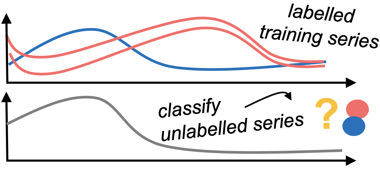
Univariate time series classification

In univariate time series classification, we have a single time series variable and an associated label for multiple instances. The goal is to find a classifier that can learn the relationship between the time series and labels, and accurately predict the label of a new, unlabelled series. sktime provides time series classification algorithms and tools for building composite machine learning models.

The basic workflow

1. Specify data
2. Specify task: Which variable is the target variable, which ones are features?
3. Specify model
4. Fit
5. Predict

Data

To find other datasets, go to: http://timeseriesclassification.com/dataset.php

from warnings import simplefilter

simplefilter(action="ignore", category=FutureWarning)

UCR UEA Dataset (documentation)

Load dataset from UCR UEA time series archive.

Downloads and extracts dataset if not already downloaded. Data is assumed to be in the standard .ts format: each row is a (possibly multivariate) time series. Each dimension is separated by a colon, each value in a series is comma separated. For examples see sktime.datasets.data.tsc. ArrowHead is an example of a univariate equal length problem, BasicMotions an equal length multivariate problem.

import matplotlib.pyplot as plt
import numpy as np
from sktime.datasets import load_UCR_UEA_dataset
from sktime.datatypes import convert

inputs, targets = load_UCR_UEA_dataset("ItalyPowerDemand", return_X_y=True)

see(inputs.head(3), 'Inputs before converting to NumPy 3D')

Inputs before converting to NumPy 3D

	dim_0
0	0 -0.71 1 -1.18 2 -1.37 3 -1.59 4 -1.47 5 -1.37 6 -1.09 7 0.05 8 0.93 9 1.09 10 1.28 11 0.96 12 0.61 13 0.01 14 -0.65 15 -0.27 16 -0.21 17 0.61 18 1.37 19 1.46 20 1.05 21 0.58 22 0.17 23 -0.27 dtype: float64
1	0 -0.99 1 -1.43 2 -1.58 3 -1.61 4 -1.63 5 -1.38 6 -1.02 7 -0.36 8 0.72 9 1.20 10 1.12 11 1.05 12 0.79 13 0.46 14 0.49 15 0.56 16 0.61 17 0.31 18 0.26 19 1.10 20 1.05 21 0.69 22 -0.05 23 -0.38 dtype: float64
2	0 1.32 1 0.57 2 0.20 3 -0.09 4 -0.18 5 -0.27 6 -0.09 7 -1.40 8 -1.12 9 -0.74 10 0.01 11 -0.09 12 0.01 13 -0.46 14 -0.55 15 -0.74 16 -0.74 17 -0.74 18 -1.12 19 -0.46 20 0.48 21 2.35 22 2.26 23 1.60 dtype: float64

inputs = convert(inputs, from_type="nested_univ", to_type="numpy3D")

This data: - 1,096 different individuals' records - 1 variable - for 24 time points

pretty(inputs.shape, 'inputs.shape')

inputs.shape
(1096, 1, 24)

# binary target variable
pretty(np.unique(targets), 'np.unique(targets)')

np.unique(targets)
['1', '2']

labels, counts = np.unique(targets, return_counts=True)
fig, ax = plt.subplots(1, figsize=plt.figaspect(0.25))
for label in labels:
    ax.plot(inputs[targets == label, 0, :][0], label=f"class {label}")
ax.set(ylabel="Scaled distance from midpoint", xlabel="Index");

Train-test split

from sklearn.model_selection import train_test_split

train_in, test_in, train_out, test_out = train_test_split(inputs, targets)

Model specification

Find out more about ROCKET:

• Repo: https://github.com/angus924/rocket
• Blog post: https://pub.towardsai.net/rocket-fast-and-accurate-time-series-classification-f54923ad0ac9

from sktime.classification.kernel_based import RocketClassifier
classifier = RocketClassifier()

Fitting

%%time
classifier.fit(train_in, train_out)

RocketClassifier()

In a Jupyter environment, please rerun this cell to show the HTML representation or trust the notebook.
On GitHub, the HTML representation is unable to render, please try loading this page with nbviewer.org.

The X here is panel data with time index data for multiple features. All SKTime fit methods need this format for their X input.

classifier.fit?

Signature: classifier.fit(X, y)
Docstring:
Fit time series classifier to training data.

Parameters
----------
X : 3D np.array (any number of dimensions, equal length series)
        of shape [n_instances, n_dimensions, series_length]
    or 2D np.array (univariate, equal length series)
        of shape [n_instances, series_length]
    or pd.DataFrame with each column a dimension, each cell a pd.Series
        (any number of dimensions, equal or unequal length series)
    or of any other supported Panel mtype
        for list of mtypes, see datatypes.SCITYPE_REGISTER
        for specifications, see examples/AA_datatypes_and_datasets.ipynb
y : 1D np.array of int, of shape [n_instances] - class labels for fitting
    indices correspond to instance indices in X

Returns
-------
self : Reference to self.

Notes
-----
Changes state by creating a fitted model that updates attributes
ending in "_" and sets is_fitted flag to True.
File:      ~/opt/anaconda3/envs/time_series_projects/lib/python3.10/site-packages/sktime/classification/base.py
Type:      method

Prediction

predictions = classifier.predict(test_in)

Evaluation

from sklearn.metrics import accuracy_score

accuracy_score(test_out, predictions)

0.9708029197080292

Classifiers in SKTIme

from sktime.registry import all_estimators

all_estimators("classifier", return_names=False)

[sktime.classification.kernel_based._arsenal.Arsenal,
 sktime.classification.dictionary_based._boss.BOSSEnsemble,
 sktime.classification.deep_learning.cnn.CNNClassifier,
 sktime.classification.interval_based._cif.CanonicalIntervalForest,
 sktime.classification.feature_based._catch22_classifier.Catch22Classifier,
 sktime.classification.compose._pipeline.ClassifierPipeline,
 sktime.classification.compose._column_ensemble.ColumnEnsembleClassifier,
 sktime.classification.compose._ensemble.ComposableTimeSeriesForestClassifier,
 sktime.classification.dictionary_based._cboss.ContractableBOSS,
 sktime.classification.interval_based._drcif.DrCIF,
 sktime.classification.dummy._dummy.DummyClassifier,
 sktime.classification.distance_based._elastic_ensemble.ElasticEnsemble,
 sktime.classification.deep_learning.fcn.FCNClassifier,
 sktime.classification.feature_based._fresh_prince.FreshPRINCE,
 sktime.classification.hybrid._hivecote_v1.HIVECOTEV1,
 sktime.classification.hybrid._hivecote_v2.HIVECOTEV2,
 sktime.classification.dictionary_based._boss.IndividualBOSS,
 sktime.classification.dictionary_based._tde.IndividualTDE,
 sktime.classification.distance_based._time_series_neighbors.KNeighborsTimeSeriesClassifier,
 sktime.classification.deep_learning.lstmfcn.LSTMFCNClassifier,
 sktime.classification.deep_learning.mlp.MLPClassifier,
 sktime.classification.dictionary_based._muse.MUSE,
 sktime.classification.feature_based._matrix_profile_classifier.MatrixProfileClassifier,
 sktime.classification.early_classification._probability_threshold.ProbabilityThresholdEarlyClassifier,
 sktime.classification.distance_based._proximity_forest.ProximityForest,
 sktime.classification.distance_based._proximity_forest.ProximityStump,
 sktime.classification.distance_based._proximity_forest.ProximityTree,
 sktime.classification.feature_based._random_interval_classifier.RandomIntervalClassifier,
 sktime.classification.interval_based._rise.RandomIntervalSpectralEnsemble,
 sktime.classification.deep_learning.resnet.ResNetClassifier,
 sktime.classification.kernel_based._rocket_classifier.RocketClassifier,
 sktime.classification.distance_based._shape_dtw.ShapeDTW,
 sktime.classification.shapelet_based._stc.ShapeletTransformClassifier,
 sktime.classification.feature_based._signature_classifier.SignatureClassifier,
 sktime.classification.compose._pipeline.SklearnClassifierPipeline,
 sktime.classification.feature_based._summary_classifier.SummaryClassifier,
 sktime.classification.interval_based._stsf.SupervisedTimeSeriesForest,
 sktime.classification.feature_based._tsfresh_classifier.TSFreshClassifier,
 sktime.classification.deep_learning.tapnet.TapNetClassifier,
 sktime.classification.dictionary_based._tde.TemporalDictionaryEnsemble,
 sktime.classification.interval_based._tsf.TimeSeriesForestClassifier,
 sktime.classification.kernel_based._svc.TimeSeriesSVC,
 sktime.classification.dictionary_based._weasel.WEASEL,
 sktime.classification.compose._ensemble.WeightedEnsembleClassifier]

But can I not just use scikit-learn?

In principle, yes, but may not be as powerful as dedicated time series classification algorithms ...

See our previous tutorial from the PyData Amsterdam 2020 for more details: https://github.com/sktime/sktime-tutorial-pydata-amsterdam-2020

Compare algorithms from sktime and scikit-learn!

from sklearn.neighbors import KNeighborsClassifier
from sklearn.pipeline import make_pipeline
from sktime.transformations.panel.reduce import Tabularizer

Tabularizer() converts panel data to cross-sectional data - this makes it possible to use other classifiers such as SKLearn models with the data - previously the data had been formatted for use with SKTime specifically - The difference in classifiers is that SKTime's classifiers are dedicated time series classifiers rather than just generic models for classification

classifier = make_pipeline(Tabularizer(), 
						   KNeighborsClassifier(n_neighbors=1, 
												metric="euclidean"))

classifier.fit(train_in, train_out)

Pipeline(steps=[('tabularizer', Tabularizer()),
                ('kneighborsclassifier',
                 KNeighborsClassifier(metric='euclidean', n_neighbors=1))])

In a Jupyter environment, please rerun this cell to show the HTML representation or trust the notebook.
On GitHub, the HTML representation is unable to render, please try loading this page with nbviewer.org.

predictions = classifier.predict(test_in)

accuracy_score(test_out, predictions)

0.9817518248175182

Advanced Model Building and Composition

• Pipelining
• Ensembling
• Tuning
• Reduction

Pipelining

Check out the tsfresh package for automatic feature extraction: https://tsfresh.readthedocs.io/en/latest/

from sklearn.ensemble import RandomForestClassifier
from sklearn.pipeline import make_pipeline
from sktime.transformations.panel.tsfresh import TSFreshFeatureExtractor

# %%time
# classifier = make_pipeline(TSFreshFeatureExtractor(disable_progressbar=True,
# 												   show_warnings=False),
# 						   RandomForestClassifier(),)

# classifier.fit(train_in, train_out)

# predictions = classifier.predict(test_in)

# accuracy_score(test_out, predictions)

---

| Top | SciKit-Learn Way | SKTime Way | Multivariate | Panel Data | SKLearn & SKTime | Univariate Forecasting | Advanced Workflow | Forecasting with Exogeneous | Building a Forecaster | Time Series Classification | Time Series Regression |
Time Series Regression

The basic workflow

import matplotlib.pyplot as plt
from sklearn.model_selection import train_test_split
from sktime.datasets import load_UCR_UEA_dataset

Find out more about the dataset here: https://zenodo.org/record/3902673#.YXqxNy8w3UI

X, y = load_UCR_UEA_dataset(name="ChlorineConcentration", return_X_y=True)
print(X.shape, y.shape)

X_train, X_test, y_train, y_test = train_test_split(X, y)

fig, ax = plt.subplots(1)
ax.hist(y)
ax.set(xlabel="target variable (bins)", ylabel="frequency");

# fig, ax = plt.subplots(1, figsize=plt.figaspect(0.25))
# for i in range(5):
#     ax.plot(X_train)

from sklearn.ensemble import RandomForestRegressor
from sklearn.metrics import mean_squared_error
from sklearn.pipeline import make_pipeline
from sktime.transformations.panel.rocket import Rocket

regressor = make_pipeline(Rocket(), RandomForestRegressor())

%%time
regressor.fit(train_in, train_out)

Pipeline(steps=[('rocket', Rocket()),
                ('randomforestregressor', RandomForestRegressor())])

In a Jupyter environment, please rerun this cell to show the HTML representation or trust the notebook.
On GitHub, the HTML representation is unable to render, please try loading this page with nbviewer.org.

# predictions = regressor.predict(test_in)
# mean_squared_error(test_out, predictions)

Reducing forecasting to time series

import numpy as np
from sktime.datasets import load_airline
from sktime.forecasting.compose import make_reduction
from sktime.forecasting.model_selection import temporal_train_test_split
from sktime.utils.plotting import plot_series

data = load_airline()
horizon = np.arange(12) + 1
training, testing = temporal_train_test_split(data, fh=horizon)

Must specify that this is a time-series regressor rather than a tabular regressor, i.e. the scitype

forecaster = make_reduction(
    regressor, scitype="time-series-regressor", window_length=12)

Look up the term "scitype" in our glossary:

https://www.sktime.org/en/stable/glossary.html#term-Scientific-type

from sktime.forecasting.compose import TransformedTargetForecaster
from sktime.transformations.series.detrend import Detrender

pipe = TransformedTargetForecaster([("detrend",
									 Detrender()), ("forecast", 
													forecaster)])

%%time
pipe.fit(training)

TransformedTargetForecaster(steps=[('detrend', Detrender()),
                                   ('forecast',
                                    RecursiveTimeSeriesRegressionForecaster(estimator=Pipeline(steps=[('rocket',
                                                                                                       Rocket()),
                                                                                                      ('randomforestregressor',
                                                                                                       RandomForestRegressor())]),
                                                                            window_length=12))])

In a Jupyter environment, please rerun this cell to show the HTML representation or trust the notebook.
On GitHub, the HTML representation is unable to render, please try loading this page with nbviewer.org.

predictions = pipe.predict(horizon)

plot_series(training, testing, predictions, 
			labels=["y_train", "y_test", "y_pred"],
		   colors = ['C0', 'C1', 'C2']);

Multivariate Time Series Classification

import numpy as np
from sklearn.model_selection import train_test_split
from sklearn.pipeline import Pipeline
from sktime.classification.compose import ColumnEnsembleClassifier
from sktime.classification.dictionary_based import BOSSEnsemble
from sktime.classification.interval_based import TimeSeriesForestClassifier
from sktime.transformations.panel.compose import ColumnConcatenator

Loading Multivariate Time Series/Panel Data

The data set we use in this notebook was generated as part of a student project where four students performed four activities whilst wearing a smart watch. The watch collects 3D accelerometer and a 3D gyroscope It consists of four classes, which are walking, resting, running and badminton. Participants were required to record motion a total of five times, and the data is sampled once every tenth of a second, for a ten second period.

input_data, target_data = load_UCR_UEA_dataset("BasicMotions", return_X_y=True)
input_data = convert(input_data, from_type="nested_univ", to_type="numpy3D")

train_in, test_in, train_out, test_out = train_test_split(input_data, target_data)
pretty(train_in.shape, 'train_in.shape')
pretty(train_out.shape, 'train_out.shape')
pretty(test_in.shape, 'test_in.shape')
pretty(test_out.shape, 'test_out.shape')

train_in.shape
(60, 6, 100)

train_out.shape
(60,)

test_in.shape
(20, 6, 100)

test_out.shape
(20,)

# multi-class target variable
np.unique(train_out)

array(['badminton', 'running', 'standing', 'walking'], dtype='<U9')

Multivariate Classification

sktime offers three main ways of solving multivariate time series classification problems:

1. Concatenation of time series columns into a single long time series column via ColumnConcatenator and apply a classifier to the concatenated data,
2. Column-wise ensembling via ColumnEnsembleClassifier in which one classifier is fitted for each time series column and their predictions aggregated,
3. Bespoke estimator-specific methods for handling multivariate time series data, e.g. finding shapelets in multidimensional spaces (still work in progress).

Time Series Concatenation

We can concatenate multivariate time series/panel data into long univiariate time series/panel and then apply a classifier to the univariate data.

steps = [
    ("concatenate", ColumnConcatenator()),
    ("classify", TimeSeriesForestClassifier(n_estimators=100)),]

classifier = Pipeline(steps)

classifier.fit(train_in, train_out)
classifier.score(test_in, test_out)

1.0

Column Ensembling

We can also fit one classifier for each time series column and then aggregated their predictions. The interface is similar to the familiar ColumnTransformer from sklearn.

classifier = ColumnEnsembleClassifier(
    estimators=[
        ("TSF0", TimeSeriesForestClassifier(n_estimators=10), [0]),
        ("BOSSEnsemble3", BOSSEnsemble(max_ensemble_size=5), [3]),])

# classifier.fit(X_train, y_train)

classifier.score(X_test, y_test)

Bespoke classification algorithms

Another approach is to use bespoke (or classifier-specific) methods for multivariate time series data. Here, we try out the HIVE-COTE (version 2) algorithm in multidimensional space.

Check out the research paper: https://link.springer.com/article/10.1007%2Fs10994-021-06057-9

from sktime.classification.hybrid import HIVECOTEV2

X_train, y_train = load_UCR_UEA_dataset("BasicMotions", split="train", return_X_y=True)
X_test, y_test = load_UCR_UEA_dataset("BasicMotions", split="test", return_X_y=True)

HiveCoteV2 is current time series state of the art

classifier = HIVECOTEV2(
    stc_params={"n_shapelet_samples": 1000},
    drcif_params={"n_estimators": 25},
    arsenal_params={"n_estimators": 10},
    tde_params={"n_parameter_samples": 100},
    verbose=0,)

%%time
classifier.fit(train_in, train_out)

HIVECOTEV2(arsenal_params={'n_estimators': 10},
           drcif_params={'n_estimators': 25},
           stc_params={'n_shapelet_samples': 1000},
           tde_params={'n_parameter_samples': 100})

In a Jupyter environment, please rerun this cell to show the HTML representation or trust the notebook.
On GitHub, the HTML representation is unable to render, please try loading this page with nbviewer.org.

predictions = classifier.predict(test_in)
accuracy_score(test_out, predictions)

0.95

Building a Classifier

Check out our classifier extension template!

This is a Python file with to-do code blocks that allow you to implement your own, sktime-compatible classification algorithm.

Summary

• univariate time series classification
• time series regression
• reduction: using time series regression for forecasting
• multivariate time series classification

Useful Resources

Research and benchmarking

• For time-series classification data sets and Java-based methods, check out timeseriesclassification.com
• For a comparative benchmarking studies, check out
  • Bagnall, Anthony, et al. "The great time series classification bake off: a review and experimental evaluation of recent algorithmic advances." Data Mining and Knowledge Discovery 31.3 (2017): 606-660. and
  • Fawaz, Hassan Ismail, et al. "Deep learning for time series classification: a review." Data Mining and Knowledge Discovery 33.4 (2019): 917-963.

Deep Learning

• For deep-learning, check out sktime's companion packages: sktime-dl

---

| Top | SciKit-Learn Way | SKTime Way | Multivariate | Panel Data | SKLearn & SKTime | Univariate Forecasting | Advanced Workflow | Forecasting with Exogeneous | Building a Forecaster | Time Series Classification | Time Series Regression | Link | Link

---